שימוש בנורמות Lp שונות לקטיעת איברי Pauli

הערה: לפני שקוראים את המדריך הזה, כדאי לקרוא את המדריך Truncate Pauli terms, שמתאר את קיצוץ איברי ה-Pauli בעלי המשקל הנמוך שמובנה בשיטה backpropagate על סמך TruncationErrorBudget שהוגדר. במדריך הזה תלמדו על ארגומנט המילת מפתח p_norm של backpropagate, שאפשר להשתמש בו כדי לשנות את נורמת ה-Lp שמשמשת להערכת השגיאה שנגרמת מקיצוץ איברי ה-Pauli.

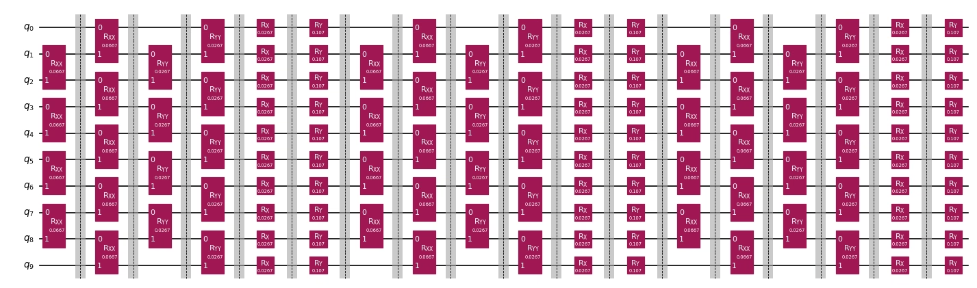
בניית מעגל לדוגמה

המדריך הזה משתמש באותו מעגל לדוגמה כמו במדריך Truncate Pauli terms:

# Added by doQumentation — installs the packages this notebook needs if they are missing
import importlib.util

_needed = {"matplotlib": "matplotlib", "qiskit": "qiskit", "qiskit_addon_obp": "qiskit-addon-obp", "qiskit_addon_utils": "qiskit-addon-utils", "rustworkx": "rustworkx"}
_missing = [pip for module, pip in _needed.items()
            if importlib.util.find_spec(module) is None]
# One at a time, so a package that fails to install does not block the others
for _pip in _missing:
    %pip install -q {_pip}
if not _missing:
    print("\u2713 All required packages are installed")

import rustworkx.generators
from qiskit.synthesis import LieTrotter
from qiskit_addon_utils.problem_generators import (
    PauliOrderStrategy,
    generate_time_evolution_circuit,
    generate_xyz_hamiltonian,
)
from qiskit_addon_utils.slicing import combine_slices, slice_by_gate_types

# Generate a linear chain of 10 qubits
num_qubits = 10
linear_chain = rustworkx.generators.path_graph(num_qubits)

# Use an arbitrary XY model
hamiltonian = generate_xyz_hamiltonian(
    linear_chain,
    coupling_constants=(0.05, 0.02, 0.0),
    ext_magnetic_field=(0.02, 0.08, 0.0),
    pauli_order_strategy=PauliOrderStrategy.InteractionThenColor,
)
# Evolve for some time
circuit = generate_time_evolution_circuit(
    hamiltonian, synthesis=LieTrotter(reps=3), time=2.0
)
# slice the circuit by gate type
slices = slice_by_gate_types(circuit)

# For visualization purposes only, recombine the slices with barriers between them and draw the resulting circuit
combine_slices(slices, include_barriers=True).draw("mpl", fold=50, scale=0.6)

נגדיר observable עבור המגנטיזציה הכוללת:

from qiskit.quantum_info import SparsePauliOp

obs = SparsePauliOp.from_sparse_list(
    [("Z", [i], 1.0) for i in range(num_qubits)], num_qubits=num_qubits
)

לצורך השוואה, נחשב את ערך התצפית המדויק:

from qiskit.primitives import StatevectorEstimator

estimator = StatevectorEstimator()
job = estimator.run([(circuit, obs)])
res = job.result()
exact_exp = res[0].data.evs
print(exact_exp)

9.318197859862146

שימוש בנורמת L1

כברירת מחדל, וכפי שכבר ראיתם במדריך Truncate Pauli terms, p_norm=1, כלומר השגיאה מוערכת כך:

$$|\langle\psi|\Delta|\psi\rangle| \leq \sum_{P\in\mathcal{T}} |c_P|$$

כאשר $\psi$ הוא המצב הקוונטי, $\Delta$ הוא ההפרש האמיתי בין ה-observable המדויק לקטום (שאינו ידוע), $\mathcal{T}$ היא קבוצת איברי ה-Pauli שקוצצו, ו-$c_P$ הוא המקדם של איבר ה-Pauli. אי-השוויון הזה הוא חסם עליון קפדני אבל רופף מאוד ברוב התרחישים. במדריך הזה מבצעים backpropagation לשש פרוסות של המעגל לדוגמה, עם שגיאה קבועה של 0.001 לכל פרוסה. את הערך הזה יש להבין כתקציב בתוך ה-p_norm הנתון.

from qiskit_addon_obp.utils.truncating import setup_budget

l1_truncation_error_budget = setup_budget(max_error_per_slice=0.001, p_norm=1)
print(l1_truncation_error_budget)

TruncationErrorBudget(per_slice_budget=[0.001], max_error_total=inf, p_norm=1)

from qiskit_addon_obp import backpropagate

max_slices = 6
l1_bp_obs, l1_remaining_slices, l1_metadata = backpropagate(
    obs,
    slices[-max_slices:],
    truncation_error_budget=l1_truncation_error_budget,
)
l1_reduced_circuit = combine_slices(
    slices[:-max_slices] + l1_remaining_slices
)
print(
    f"Backpropagated {max_slices - len(l1_remaining_slices)} circuit slices."
)
print(
    f"New observable contains {len(l1_bp_obs)} terms and {len(l1_bp_obs.group_commuting(qubit_wise=True))} commuting groups."
)

Backpropagated 6 circuit slices.
New observable contains 116 terms and 10 commuting groups.

עכשיו אפשר לחשב את ערך התצפית של ה-observable אחרי ה-backpropagation, וכן את השגיאה ביחס לייחוס המדויק:

estimator = StatevectorEstimator()
job = estimator.run([(l1_reduced_circuit, l1_bp_obs)])
res = job.result()
l1_exp = res[0].data.evs
l1_error = exact_exp - l1_exp
print(l1_exp, l1_error)

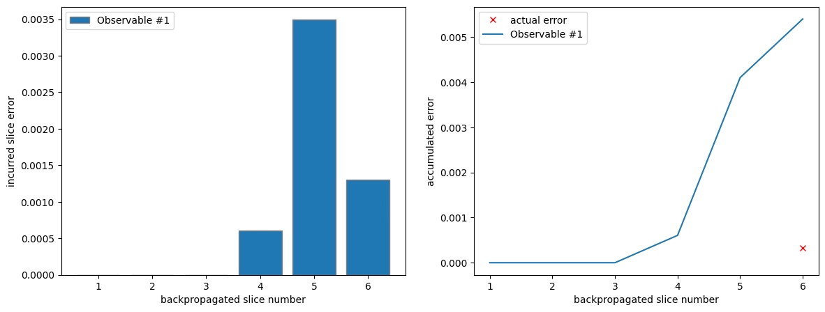
9.317869899338842 0.00032796052330397174

לבסוף, אפשר להציג בגרף את השגיאה שנגרמה במהלך ה-backpropagation של כל פרוסה, וגם את השגיאה המצטברת. השגיאה המצטברת היא סכום שגיאות הפרוסות. אפשר לראות שהשגיאה המצטברת היא חסם עליון רופף מאוד לשגיאה האמיתית.

from matplotlib import pyplot as plt
from qiskit_addon_obp.utils.visualization import (
    plot_accumulated_error,
    plot_slice_errors,
)

fig, axes = plt.subplots(1, 2, figsize=(14, 5))
axes[1].plot([6], [l1_error], "x", color="red", label="actual error")
plot_slice_errors(l1_metadata, axes[0])
plot_accumulated_error(l1_metadata, axes[1])

שימוש בנורמת L2

אפשר לטעון שנורמת L2 מקרבת טוב יותר את השגיאה שנגרמה מאשר נורמת L1. זה בגלל שאפשר להניח שהמצב הקוונטי $|\psi\rangle$ נדגם מאנסמבל אקראי של Haar, ובמקרה כזה השגיאה שנגרמת מתפלגת עם תוחלת שואפת לאפס ושונות שאפשר לחסום בקירוב באמצעות נורמת L2:

$$|\langle\psi|\Delta|\psi\rangle| \lesssim \left( \sum_{P\in\mathcal{T}} |c_P|^2 \right)^{1/2}$$

החסם אמנם אינו קפדני, אבל הוא יופר רק במקרים פתולוגיים. שוב נבצע backpropagation לשש פרוסות של המעגל לדוגמה, עם שגיאה מרבית של 0.001 לכל פרוסה (הפעם מפורשת לפי נורמת L2).

l2_truncation_error_budget = setup_budget(max_error_per_slice=0.001, p_norm=2)
print(l2_truncation_error_budget)

TruncationErrorBudget(per_slice_budget=[0.001], max_error_total=inf, p_norm=2)

max_slices = 6
l2_bp_obs, l2_remaining_slices, l2_metadata = backpropagate(
    obs,
    slices[-max_slices:],
    truncation_error_budget=l2_truncation_error_budget,
)
l2_reduced_circuit = combine_slices(
    slices[:-max_slices] + l2_remaining_slices
)
print(
    f"Backpropagated {max_slices - len(l2_remaining_slices)} circuit slices."
)
print(
    f"New observable contains {len(l2_bp_obs)} terms and {len(l2_bp_obs.group_commuting(qubit_wise=True))} commuting groups."
)

Backpropagated 6 circuit slices.
New observable contains 84 terms and 6 commuting groups.

שוב נחשב את ערך התצפית של ה-observable אחרי ה-backpropagation ואת השגיאה ביחס לייחוס המדויק:

estimator = StatevectorEstimator()
job = estimator.run([(l2_reduced_circuit, l2_bp_obs)])
res = job.result()
l2_exp = res[0].data.evs
l2_error = exact_exp - l2_exp
print(l2_exp, l2_error)

9.317829770853422 0.00036808900872387085

הצגת השגיאות שנגרמו בכל פרוסה והשגיאה המצטברת בגרף נותנת תמונה דומה לקודמת.

fig, axes = plt.subplots(1, 2, figsize=(14, 5))
axes[1].plot([6], [l2_error], "x", color="red", label="actual error")
plot_slice_errors(l2_metadata, axes[0])
plot_accumulated_error(l2_metadata, axes[1])

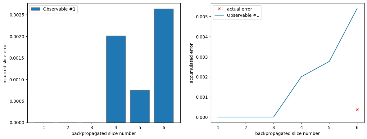
שימו לב שהשגיאה המצטברת היא שוב סכום שגיאות הפרוסות הבודדות. זהו חסם רופף נוסף בגלל אי-השוויון של Minkowski, מפני שאנחנו צריכים לחשב את החסם הזה באופן רקורסיבי:

$$|\langle\psi|\Delta_{i}|\psi\rangle| \leq |\langle\psi|\tilde{\Delta}_{i-1}|\psi\rangle| + \left( \sum_{P\in\mathcal{T_i}} |c_P|^2 \right)^{1/2} = |\langle\psi|\tilde{\Delta}_{i}|\psi\rangle|$$

כאשר האינדקס התחתון החדש $i$ מציין את איטרציית הפרוסה הנוכחית, כך ש-$\Delta_i$ היא השגיאה האמיתית באיטרציית ה-backpropagation ה-$i$, ‏$\tilde{\Delta}_{i-1}$ היא שגיאת הקיצוץ המקורבת מאיטרציה $i-1$, ו-$\mathcal{T}_i$ היא קבוצת איברי ה-Pauli שקוצצו באיטרציה $i$.