אלכסון קוונטי מבוסס דגימות מאוחדות של המילטוניאן גרעיני
הערכת שימוש: 32 שניות על מעבד Nighthawk r2 (שימו לב: זו הערכה בלבד. זמן הריצה שלכם עשוי להשתנות.)
תוצאות למידה
-
למדו כיצד המילטוניאן של מודל הקליפות הגרעיני, המוצג בטבלאות בבסיס מצומד- של אורביטלים, הופך להמילטוניאן של Qubits בסכמת , שבה Qubit אחד הוא מצב חלקיק-יחיד אחד.
-
בנו אנסץ קבוע ולא וריאציוני של עירורים, שזוויותיו נגזרות מתורת ההפרעות מסדר שני, כך שאין לולאת אופטימיזציה קלאסית.
-
השוו בין עירורי Qubits לעירורים פרמיוניים ומדדו כיצד הבחירה משפיעה על עומק שני-ה-Qubits של האנסמבל.
-
הריצו שחזור קונפיגורציות עקבי-עצמית באמצעות
qiskit-addon-sqdכאשר הגדלים השמורים הם מספרי הנוקלאונים, וזוגיות, ולא מספרי האלקטרונים והספין. -
החילו זרימת עבודה אחת מבעיה של 24 Qubits שאפשר לבדוק במדויק על בעיה של 40 Qubits עם כמעט שני מיליון מצבי בסיס, מעבר ליכולת האלכסון המדויק של המדריך הזה.
דרישות מקדימות
לפני שמתחילים, עברו על הנושאים הבאים:
-
אלכסון קוונטי מבוסס דגימות של המילטוניאן כימי, המקביל האלקטרוני של המדריך הזה.
-
קוונטיזציה שנייה ומיפוי ג'ורדן-וינגר.
רקע
מודל הקליפות הגרעיני מתייחס לגרעין כאל מספר קטן של נוקלאונים ולנטיים שנעים בקבוצה קטנה של אורביטלים חד-חלקיקיים מעל ליבה אינרטית, ומקיימים אינטראקציה דרך כוח דו-גופי אמפירי שהותאם לספקטרום שנמדד. הוא נמצא בשימוש נרחב בחקר מבנה גרעיני באנרגיות נמוכות. עלות החישוב שלו קומבינטורית: הבסיס הוא כל הדרכים לפזר את הפרוטונים והנויטרונים הוולנטיים על המצבים הזמינים, והצמיחה הזו מגבילה את מרחבי המודל הנגישים לאלכסון מדויק.
אלכסון קוונטי מבוסס דגימות מאוחדות (SQD מאוחד) [1] מפצל את הבעיה לשניים. מעגל קוונטי משמש רק כדי להציע אילו מצבי בסיס חשובים. הוא נמדד בבסיס החישובי, וכל מחרוזת ביטים שנמדדה מגדירה דטרמיננטת סלייטר אחת. לאחר מכן ההמילטוניאן נבנה ומאולכסן באופן קלאסי במרחב הנפרש על ידי הדטרמיננטות האלה. מכיוון שהשלב הקלאסי הוא אלכסון מדויק בתוך תת-מרחב, הוא מחזיר חסם עליון וריאציוני לאנרגיית מצב היסוד האמיתית, והחסם יכול רק לרדת ככל שמוסיפים דטרמיננטות.
חלוקת העבודה הזו הופכת את השיטה לעמידה בפני רעש, עם הגבלה חשובה. רעש משנה אילו דטרמיננטות המעגל מציע. הוא אינו נכנס להמילטוניאן הקלאסי, ולכן אינו יכול להזיז את הערך העצמי של תת-מרחב נתון: דגימה שמפרה גודל שמור נזרקת או מתוקנת, ודגימה ששורדת היא וקטור בסיס לגיטימי לא משנה כיצד נוצרה. לכן הרעש עולה לכם באיכות התת-מרחב ולא בנכונות, והמספר שאתם מדווחים הוא חסם עליון בכל מקרה.
מבנה גרעיני מספק כמה מספרים קוונטיים מדויקים לסינון דגימות. דטרמיננטה פיזיקלית חייבת לשאת את המספר הנכון של פרוטונים ולנטיים וגם את המספר הנכון של נויטרונים ולנטיים, את ההיטל הנכון של התנע הזוויתי הכולל , ואת הזוגיות הנכונה. אפשר לבדוק כל אחד מהם בבדיקה של מספרים שלמים על מחרוזת ביטים. שיעור הדגימות שנדחות תלוי באילוץ ובמרחב המודל.
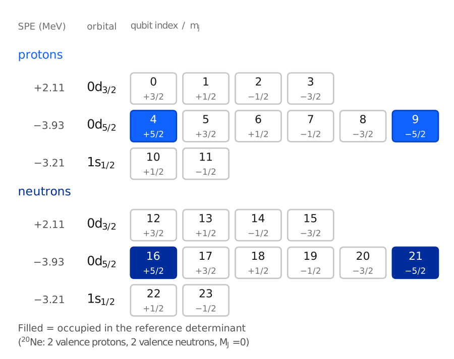
כל Qubit הוא מצב חלקיק-יחיד אחד בסכמת , , ו- פירושו תפוס. הרגיסטר משתמש בסדר קבוע: קודם פרוטונים, אחר כך נויטרונים; בתוך סוג חלקיק, אורביטלים לפי סדר הקובץ; בתוך אורביטל, יורד. שני חצאי מחרוזת הביטים הם אפוא קונפיגורציית הפרוטונים וקונפיגורציית הנויטרונים. זו החלוקה לשני חלקים שכלי העיבוד שלאחר המדידה של SQD מאוחד מצפים לה.
זרימת העבודה
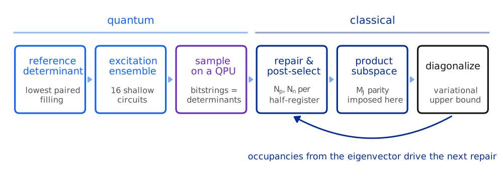
שני שלבים בתרשים מטפלים בסימטריות הגרעיניות.
תיקון וסינון לאחר הדגימה מטפלים בדגימות שהושפעו מרעש החומרה. מספרי הנוקלאונים בשני חצאי הרגיסטר הם משקלי המינג, ולכן qiskit-addon-sqd מטפל בהם ישירות: recover_configurations מתקן מחרוזת ביטים פגומה על ידי היפוך הביטים הכי פחות עקביים עם ההערכה הנוכחית של התפוסות הממוצעות של האורביטלים, במקום לזרוק את הדגימה.
תת-המרחב המכפלתי מכניס את . מכיוון ש- מצמד בין שני החצאים, הוא אינו תכונה של אף אחד מהם, ולכן אסור להשתמש בו כדי לסנן דגימות שלמות: מחרוזת ביטים שחצי הפרוטונים וחצי הנויטרונים שלה תקינים עדיין תורמת שתי חצאי-קונפיגורציות טובות גם כאשר הכולל שלה שגוי. תת-המרחב נפרש אפוא על ידי כל מכפלה של קונפיגורציית פרוטונים שנדגמה עם קונפיגורציית נויטרונים שנדגמה, תוך שמירה על המכפלות שנוחתות במקטע היעד של וזוגיות. זוהי בניית תת-המרחב של SQD מאוחד, והיא אומרת שכמה אלפי מחרוזות ביטים יכולות לפרוש תת-מרחב גדול בהרבה ממספר הדגימות.
שתי משוואות מנחות
ההמילטוניאן של מודל הקליפות הוא איבר חד-גופי ועוד אינטראקציה דו-גופית,
כאשר מסמנים מצבים בסכמת ו- לפרוטון, לנויטרון. אינטראקציות אמפיריות כמו USDA [2] ו-GXPF1 [3] אינן מוצגות בטבלאות בסכמת אלא בבסיס המצומד-, כאיברי מטריצה בין מצבים דו-גופיים מנורמלים ואנטי-סימטריים של אורביטלים . שחזור האיבר בסכמת הוא צימוד מחדש של קלבש-גורדן,
כאשר הגורמים מבטלים את מוסכמת הנרמול של המצבים שבטבלאות. כל השאר במדריך הזה בנוי על שתי המשוואות האלה.
שלוש הריצות
| גרעין | קליפה | Qubits | בסיס מותר לפי סימטריה | ניתן לבדיקה מדויקת? | |
|---|---|---|---|---|---|
| קנה מידה קטן | (2p + 2n) | 24 | 640 | כן | |
| קנה מידה גדול | (2p + 2n) | 40 | 4,000 | כן | |
| קנה מידה גדול | (4p + 4n) | 40 | 1,963,461 | לא |
הריצה בקנה מידה קטן היא הדרכה צעד אחר צעד. שתי הריצות בקנה מידה גדול משתמשות ברגיסטר של 40 Qubits: הראשונה עדיין קטנה מספיק כדי לאלכסן אותה במדויק על מחשב נייד, כך שאפשר להשוות את תוצאת החומרה להפניה מדויקת. השנייה חורגת מיכולת האלכסון המדויק של המדריך הזה.
כל ריצה כאן מתבצעת על QPU. זו בחירה שנעשתה למדריך הזה ולא דרישה של השיטה: שלוש הריצות חולקות Backend ותקציב שערים משותפים כדי שתוכלו להשוות את הביצועים שלהן בגדלי בעיה שונים.
דרישות
התקינו את החבילות הבאות לפני שמתחילים:
-
Qiskit SDK גרסה 2.0 ומעלה (
pip install qiskit) -
qiskit-ibm-runtimev0.40 or later (pip install qiskit-ibm-runtime) -
תוסף SQD גרסה 0.12 ומעלה (
pip install qiskit-addon-sqd) -
NumPy, SciPy ו-Matplotlib (
pip install numpy scipy matplotlib)
תזדקקו גם לחשבון IBM Quantum® עם פרטי גישה שנשמרו באופן מקומי, וגישה ל-QPU עם 40 Qubits לפחות.
לא נדרשת חבילת סימולטור, ואין צורך להוריד קובצי נתונים. שני קובצי האינטראקציה שהמדריך הזה משתמש בהם מוטמעים בתא ההגדרה הבא ונכתבים לתיקייה זמנית כשמריצים אותו.
הגדרה
החלק הזה מייבא את הכלים ומגדיר את פונקציות העזר של מודל הקליפות שזרימת העבודה צריכה, לפי הסדר שבו זרימת העבודה משתמשת בהן. הפיזיקה שמאחורי כל אחת מהן נגזרת בנספח; ההערות מתארות את תפקידה של כל פונקציה בזרימת העבודה.
קודם נפרקים שני קובצי אינטראקציה. שניהם קבוצות פרמטרים שפורסמו, והם מוטמעים כאן כדי שה-Notebook יהיה עצמאי: usda.snt הוא ההמילטוניאן USDA של קליפת [2] ו-gxpf1.snt הוא ההמילטוניאן GXPF1 של קליפת [3].
# Added by doQumentation — installs the packages this notebook needs if they are missing
import importlib.util

_needed = {"matplotlib": "matplotlib", "numpy": "numpy", "qiskit": "qiskit", "qiskit_addon_sqd": "qiskit-addon-sqd", "qiskit_ibm_runtime": "qiskit-ibm-runtime", "scipy": "scipy"}
_missing = [pip for module, pip in _needed.items()
            if importlib.util.find_spec(module) is None]
# One at a time, so a package that fails to install does not block the others
for _pip in _missing:
    %pip install -q {_pip}
if not _missing:
    print("\u2713 All required packages are installed")
from __future__ import annotations

import base64
import gzip
import itertools
import tempfile
from dataclasses import dataclass
from functools import lru_cache
from math import factorial, sqrt
from pathlib import Path

import matplotlib.pyplot as plt
import numpy as np

from qiskit import QuantumCircuit
from qiskit.circuit.library import PauliEvolutionGate
from qiskit.quantum_info import Operator, SparsePauliOp
from qiskit.transpiler.preset_passmanagers import generate_preset_pass_manager
from qiskit_addon_sqd.configuration_recovery import recover_configurations
from qiskit_addon_sqd.counts import bit_array_to_arrays
from qiskit_addon_sqd.subsampling import postselect_by_hamming_right_and_left
from qiskit_ibm_runtime import QiskitRuntimeService, SamplerV2

from scipy.linalg import eigh

_USDA_SNT_GZ = (
    "H4sIAI5wqWoC/4WY224bRwyG7/UU9F0CONsZco5AUyBuC/QmQNG06KWhWGql1LYMy+kJefiOTrucGXJrQAgsf5nl8ecOr+CX"
    "D9+9g/0K9pv1/T389rx7gPLrsH+Cz/vVctg+vgAsrgB+HeDdAD9t7zYv6+dr+DDA+z8223/X17B8XMFN+ev9+m+4ed799XjA"
    "f9z8sy/4+s8BvoWYrsEERwbhFRqTXi+uCvOwW63vYf+0vFvDAgDo/AFIh8/hK7DH30354Omvb8o3V8c/vIUnMKtboK/wiGKF"
    "+gnFEfVn9PQUe8bthNIRtftbsGfUtQbAGXUFfawM8K0BF9SP6MWA0BpwQcMRvRhwBSX86+fl3ct2d4jq4+eHa3hYv2x2q7fX"
    "AJuPy+fb3cP69+Uh4luAT8djv95++eGV/fj6y6dvFudnmcX4lGOoBmttNOVncTL2FLs3NGT0l++ndJTv0cR8/t6NUanP8WMI"
    "6nPC6C8/5wp+vnn//QLOP9ank3k2wRszkDn/Zwv15xiv41l2SDmjhuEFM4PJ0QkYcgzM4A1Jp1GDkcvtaWMAR9tosAa9huHk"
    "AtoUBYwaF8hGarAxOywgxnoeN+Se2smF4H3QMPZQ653XMJpOi6GyrcLcZJtzLgoYcdsOyXKibV1Aom0fikJO0VLUMDeW3kAl"
    "qQLWpd66qGE02eZ9lXqSPD3UWyl5DeOeGnINJnmaUggCVrtgh2DJNm3fVy8WF3LSMFa9hYga5iYX0IQsYK2nmTpJkoq81Acy"
    "jLTTnPEaxqo3JGcbvZMeGnJVbw6mf2cUqcIsO80nFdOFq8JoSlY+Zb7FfNNZlnw2PqOE8SL3PtlSJhJGXGqsDRjbh4bmocWy"
    "oiIxSxjv09JYgaxlGLZxA9EFFOImuIBt3EB04TK3Z5S8wizrrFCJQ4Xpgl9hzDYbu0LCNm6HzkJHweUkYazITalyF7NjGAnh"
    "FZJFQniFZFHnqWgbdZ6qtoX50VZhvEJ81TJe7AUcQozH8yQMJ8ymUS07jLin6LXT3FRIhmwSTmtbJpEjr2AsvM7E1ra+ZaiM"
    "NoxewZinBlPQTmPJyikn7TQ2630SbWuz4CLlwzuGhCHPqbUmRZQwpkiBDn1vsoQ55oKjbEvNNVgbXls0WvA0NKnPpku91Fkx"
    "pahhXPDJtxVCQkBcMtJD27I8VJGAhWYYlVuZzc5e+jSIZWnLa57nOQ1iWZY+jSE3GP5/QIKi5E1Agqi9BbMZiUjEWNwChqKq"
    "KTZY11ku5ca2Pqc4YKk1o2DstBjJC1htW2nAgEZ4aDdPvQmmmLeY4tWFt9Y3VAdlpW+oDcpa3zpM1jdUB2XV9agOyqrrcWZQ"
    "sq7vMMffBseux5l5yjoLZ+Yp6yzU5mmt5DgzT5mSozZPoVIknJmnTJFQHZRV12OrlvpFQFbycoGKOWiYfl9QlXySGtSUvL9W"
    "VJi/YG4grC4CmuCX6CZrKUsY64UyJolCQoZJqWeKhDOCzxQJNcGXbZMEX7EtzF+gvCI1npxjmKaW5Q06ewVjOY0u2+Y0kt5D"
    "JhlETS2P+5CqyIMYkCI1NK50SO3TarSR2qfVaKOZPmXjg2beVJmS01zqp/CSmvoqvNSOD/kaS+qUoSGaTM2yz83fdjtMvsZy"
    "xOv7N44Fff/GT5q5tXWYfB3jWND3b9yumUvK5SQnvK6w/VuHyfu3DpP3bx0m7984FvT9W4fJ+zceWq/v3zpM3r9xLOj7tw6T"
    "928X053QgGz/1mHy/u3yZ8lTtn/jWND3b74NiDx2vRbeep56Lbz1oPRaeOv9G0dmxofXPK33bx0m798C1B9RuP4DPJ0WcLAa"
    "AAA="
)

_GXPF1_SNT_GZ = (
    "H4sIAI5wqWoC/4WcQY8dtw3H7/kU41sCeF8lUqKkQw9NgbaXoEHQQ26BkdiIEWdt2E6L9tNXb9+ORIn8PwdZILB/S3I4IsW/"
    "ZiYvjr//+P3f4nG8ef/x+PDm4dOvr9+9++rF8d3l+Mf7x99fvTz+dTn++fnTH7/1//z28pfL8e3H9/95fHm8evzl+lffvf3f"
    "H59e/fb26L9zHN//+t9Pl+OH1/++HH89JL88gkQO8esfvjm+phDomyvW//39/S+v3x2fPrz6+fVX/dfS889B4fpz/aN43P7p"
    "f3Bw/ynH8fD0Zy+uf/fn48MR3vxU/kRXlp7Z+PzDiqUnNn74iW8sb3azYvm0m29s2uxGxabTbryx2cZ7nGzu7KOKV2y8g5Un"
    "dsZbbLyDLafd53irjXew9bR7jffF8fbx8+uPr37+/Pb941dPv3P93ZH4W/If6kUohXCm+Jbmh3yR0jicybwl9CFeuFILy908"
    "HtIlcrlZyCNJ2q6MdGi7ZVy4tlvHJS52Y71FnHp8D+HCIYTlQuYFhdsv0yVxzZB6vsxwaZwJUumkIjWB1POdDhcqlR2KVo85"
    "SoDU8NgdNodiZevqMUqB1LCVWsO2ZMQlyYs+bXEFk4m5bMJJlVgSpGjaouhQvFKxUIbUjIvI85hWW4FNvubyDnMxMkFKRc8V"
    "Uml65OhQW1x9fe3XOAtsZPXJ36TIX18SaoQUnysnZsHUXPfcKqTyaSu36FHbWg0tN0jxWIXEAVLzbqcqkMpj3T8lwlBp9RhD"
    "qpAaHpnzni9nRXPh6lDbysmJBVLzDtU71KztnDxqW1+JhDaKnTtUa4DUzH00Hp0VXQMHSM3c16irlpf7GEcN1dogpfpEDpAa"
    "WRUOBKl0UqkIQ2qs+5IYU6OvthbFodIaF6/9i51VeF0TLZSN2lfh9T729utQOqtXKi/dl/21mihhW+M+BpIKqblypDWHSntc"
    "mSA1O3nMe+6dHp0DEaRmXCU0h9p7dOYCqVm1MehOnvy7nWphSKnuu+Q++X2Ca4uQGrYkxp3yMkFLL0ygavPovmR64dhFY5QM"
    "KVK1XRxqX4UydlHCXU44hY1ydndKuUBK11BzqH1NNOKNMvt27PMXVUWBemSqCVIjrr4nYFtzTSQJkJp3O7se09p9YygCKVL7"
    "UN4opx5DNnE5q5AlerZ2jyExpEYmggTtMYFrzC1Bak58jetGeSvHenSip9ROik0m5lqdsxzjrCYhTM1uImOHYZzVPvnWjXIm"
    "0RoaKyqhjjlqiEE3uWoYHqopbT/KY0pDD+Xtx9d8lvI0n6U8zWcpT/NpQqDms5Sn+TRVoOazlKf5LOVpPk1VqPl05AI1n6U8"
    "zaepAjWfpTzNp6kKNZ/OQoGaz1Ke5rOUp/k0VaHm03mvUPOd1+esL6X5LOVpPkt5ms9SnubTVIGaz1Ke5rOUp/ks5Wk+TVWo"
    "+SzlaT69mgVqPk0VqPks5Wk+S3maT1MVaj5dPwVqPkt5mk9TFWo+S3ma77x/8z56ms9SnuazlKf5LOVpPkt5ms9SnubTVIWa"
    "z1Ke5jupfRWumk9TBWo+S3maz1Ke5rOUp/k0VaHms5Sn+XTnLVDzWcrTfJqqUPNZytN85/1z7rbSfJbyNN/5t06fUJrPUp7m"
    "OykvE7T0wgqqdmo+Mb3Q03yCO6bSfII7ptJ8gruc0nxi+pen+eROL5yaT3CXU5pPx1Sh5hNcj0rzCajHVfMJqMdV88mdesyu"
    "xwo1n+B6VJpPcD0qzSe4HpXmE1yPSvMJrkelwERVR4Waz1Ke5hNTQ3THoxO90nzFZMLTfAVnVWm+grOqNF/BWVWaTxMVar6C"
    "r1FpvgK6yar56vbja76onormu8/5ViqOrNblZH6l0NPAlRq9sKaIbaFnhis15tUuH/E1oieLK1XOTIgsz3ROap9XpQ/SJWqK"
    "bCYcKm6K4tp9iUqqzbd1j4qO+g2tpTV6sll1qLipk6fnw32/isDWPSruPborwz7x9eakKbbry6Gi7RN9nrhuHr4tPXXsVLT9"
    "vvTdKlUQ18i9Q0Wn+2ZOlYpva0yiDhXthNz69p4S+7ZG7h0q2jma+/BIIfm2RnU4VLQ9R6hG4iWryVurhorOlNbzEJr4tubk"
    "bim6e25iqbFbJY4MKfREfaXGNXKK2aF2BSapD6Oy5162yd1S5Og0iq3k5tua1WEpsus+ZO4ZS76tqU4sRc7+mAtJyL6teR8t"
    "RVbDUO9yXM2a2O6jQ5GjdCi3HKpva04dluK7J1uWGtFLjhFS6J2HlZpKhzOm0JsRK5XnmjD7Izv5av0eBd7zVb5IsVU6ffTN"
    "oQXf1peoeveNjZWaNURFZ0L8fTsX1s9hwO4eeHkOA3Z3Zct6ZOccgPAM0O91hR4ZPEcWMAPkdBWQvsdZj72xZuTRs2U95qFY"
    "a8FZHVQpy/Mhd55YbGmPew2VGB2PRvOVsNlib0orYbO1U8fi0cbF6uQhw7jUycMybYs/dSiKwGxyLB5tXEmdM5WM4lKnGLFm"
    "FFeaPTruK8ehlEcbV55n2yIwrnlOXorAuPKsxyIwrjz7l3greptzSgve+tqo2lLbcu9MQ4oiPDMpjzaueR8rUUZxqaql/T46"
    "k5WiCM9fyuNpy5uZpM9WkvfaxpS1Ndd96JKV2LflUdrW1idaKOT0HNMnTCdnT/OZvcOZv5RHG5fqAJFhXLO2WykwrtlzJkV4"
    "llMebVxp7kOUMopr7h1dSmcUl9LuxesT2z6kPOq4ttkkk7sj1/1JWWWnHvfdfVKE50LlUV+jObPqs2hO+zViytpSJ+CFSyu+"
    "LY+yttRM3gf3HH1bHmVtzR5NXZQXcI0epW1tdyh2d86a2O52F9vR6V8FUgTm1dWjjWuepZUgMK45k2cKMC6PIjD7rh6j+gpi"
    "0Y904b675/n2h3u6QteTedkoc7qy2LIeaUxpkXNAHgeV53khozOYxZb1qDpTrvAa+TxBClECvEbPlvWY5o4cA7zGNDSfFIbX"
    "6NmyHmd1SEnwGgfVJ6YKr9GzZT3KebdDZIYe5bzGQLFAj54t7XHXfDkmJ6v789r17e7iTEMrxXhmUh5tXHNmainCuObMVBOO"
    "y6MYzEyrx9MW2VMf4cC9NWlbzpmVoqytucPkIO12SsZ4/lKUtTX7V6LGsfi2phadlLa1nX89naUHc437uYnQni/nlEzWN/S8"
    "s7TVo41LvUsW9+pwqFBl79HsPYkVr/sK9GjjYnVWSzBfqjoowXx5FN+ZC6dHG5d6WybjfM15ouYE8+VRDObC1aOOa3v+WEJq"
    "Tlzb2VCRELOtbYEU47NH5dHGpd5nagzj0s+HAozLoxjMq6tHnfutHmNjblz23G/1qChra3rMOT6f3jGefRVlbamZKfR1COKa"
    "PWdS1tZcXy3mnMm3pd4IGpS1Nd9Uai0Wir6t+fxxUtrWPvu27M1MG8XJ1KMz+yqK8Vmt8mjjmn1CKmcUF88zhVIzimtOtZNi"
    "fO6rPGpbW9XGLrg50G5rfwNhUueu7swmEtI55yQ0m/RpqI3JPd15ujVtWY9TSbcxpSU8dSShAj16tk4b3r6dmUlI2/L27Ulp"
    "W7vKLFK3uByK4nI2VP19SFEJ7EOrRxvXyESr413YhPchLsssV/0dRlEJ70PKo7a1n/vWa1rLbsu8mTooa0up8tpyEd+Wep42"
    "KG1rf6su5ebkvpqztLzl3qltRSVc28ojmTM+9F2TwNm3Qgp9/eSeKnaNXFtwqH3nk1KaJE05M6ZDOdNjv9NJIvm2Zr+3lFeP"
    "EvqGnH1bM/eWMtNQvFCRHnzUlJlzXMqZYFKqHHLxbdFUFIbiu+8XWmo+50vL6R06l1u/PBO/asN8B5zAmdXTDtP7r8h+jeWL"
    "lFOPocYumti39SWq3v0iTvxdtDw9hhmUq9N6PbaqvzJyqyNeMi0nIm51LLbojgIrOUKP+l2yBj16tghrqxib1gqg0pLknfIq"
    "bdoirJqkMMNrnDNATPgaPVuE9VBv0J7HbU107V42W44eUhSjPrF4JKyHUokZxqXeTV+exAI9pCjGp/zKIwE9dO2+XSTX1vbc"
    "b6pJUYT1UOCWWw2+rdmZJkVYD1Ef0Uoi39acySdFWA9RztLVjm9LPQ0cFAENc3unJjrVsWuY0mK297EYxbrbcs7vlUfCGib3"
    "bQ/GNWffMijCGkZRDHr0w+KRsIbpnem6dnZbe9VOitTsW7e3I+e7Pgnv7tfHQxvl7O7KlvU4zu95fouUUNV21RSGFk2oHhdb"
    "ZGbf+b4cXf8nRlnb8maASVlbc+UkSnSb0hKox4eFIjNHz7c/aHydkvC6T9Lydo3Je+u8ZSdf+xsu06O2ta2vPr70W1l2W9v6"
    "UhSbPoG+kwYnSDVnTKGvqYvfv3JuDVLom2vvpOZpvh9fizHuX71jVp79vqDcG8rrJolLnecTxe8TgMLfBTDoJteOGUVntYJr"
    "5PHOVsKnUaEuJw8oE9MWA5V5e2tA9wmQrw5xQB6RrernS33VkEB1PCmKW5f7P6zudeW7TwAA"
)

DATA = Path(tempfile.mkdtemp(prefix="nuclear_sqd_"))
for name, blob in (("usda.snt", _USDA_SNT_GZ), ("gxpf1.snt", _GXPF1_SNT_GZ)):
    (DATA / name).write_bytes(gzip.decompress(base64.b64decode(blob)))

    if not (DATA / name).is_file():
        raise RuntimeError(f"{name} did not unpack to {DATA}")
מרחב המודל ורגיסטר ה-Qubits
קובץ .snt מכיל את מרחב המודל, את האנרגיות החד-חלקיקיות ואת איברי המטריצה הדו-גופיים המצומדים-. באינטראקציות התלויות במסה שבהן משתמשים כאן, השדה השלישי והרביעי בכותרת הדו-גופית מציינים את מסת הייחוס שבה הותאמה האינטראקציה ואת מעריך התלות במסה. בשני הקבצים המעריך הוא , עם ל-USDA ו- ל-GXPF1, ולכן יש לשנות את קנה המידה של איברי המטריצה שבטבלאות ב- עבור הגרעין שמחושב [2], [3]. האנרגיות החד-חלקיקיות אינן משתנות בקנה המידה. דילוג על השלב הזה משנה את אנרגיית המתאם באחוזים בודדים.
האנרגיות שלהלן הן אנרגיות ולנטיות, הנמדדות מהליבה האינרטית; הן אינן אנרגיות הפרדה ניסיוניות.
@dataclass(frozen=True)
class Orbital:
    idx: int
    n: int
    ell: int
    j2: int
    tz: int  # j2 = 2j; tz = -1 proton, +1 neutron

@dataclass(frozen=True)
class SPState:
    """One m-scheme single-particle state, i.e. one qubit."""

    orb: int
    j2: int
    mj2: int
    tz: int
    ell: int
    spe: float  # mj2 = 2 * m_j

@dataclass
class ModelSpace:
    orbitals: list
    spes: dict
    tbmes: dict
    core_z: int
    core_n: int
    mass_number: int
    a_ref: int
    mass_exponent: float
    mass_factor: float

def read_snt(path, n_protons, n_neutrons):
    """Parse a .snt interaction file, applying its mass dependence for this nucleus.

    The two-body header line is ``n_tbme  method  A_ref  exponent``.  When ``method`` is 1 the
    tabulated matrix elements are rescaled by ``(A / A_ref) ** exponent``, where A is the mass
    number of the whole nucleus -- the core plus the valence nucleons.  A is derived from the
    file's own core numbers rather than passed in, so it cannot silently disagree with the
    valence counts the rest of the workflow uses.  Single-particle energies are not rescaled.
    """
    rows = [
        ln.split("!")[0].split() for ln in Path(path).read_text().splitlines()
    ]
    rows = iter([r for r in rows if r])

    n_p_orb, n_n_orb, core_z, core_n = (int(x) for x in next(rows)[:4])
    orbitals = [
        Orbital(*(int(x) for x in next(rows)[:5]))
        for _ in range(n_p_orb + n_n_orb)
    ]

    spes = {}
    for _ in range(int(next(rows)[0])):  # "i  i  <i|H(1b)|i>"
        field = next(rows)
        spes[int(field[0])] = float(field[2])

    n_tbme, method, a_ref, exponent = next(rows)[:4]
    n_tbme, method, a_ref, exponent = (
        int(n_tbme),
        int(method),
        int(a_ref),
        float(exponent),
    )
    mass_number = core_z + core_n + n_protons + n_neutrons
    factor = (mass_number / a_ref) ** exponent if method == 1 else 1.0

    tbmes = {}
    for _ in range(n_tbme):  # "a  b  c  d  J  value"
        field = next(rows)
        tbmes[tuple(int(x) for x in field[:5])] = float(field[5]) * factor

    return ModelSpace(
        orbitals,
        spes,
        tbmes,
        core_z,
        core_n,
        mass_number,
        a_ref,
        exponent,
        factor,
    )

def m_scheme_states(ms):
    """The qubit register: protons then neutrons, orbitals in file order, m_j descending."""
    return [
        SPState(o.idx, o.j2, m2, o.tz, o.ell, ms.spes[o.idx])
        for tz in (-1, +1)
        for o in ms.orbitals
        if o.tz == tz
        for m2 in range(o.j2, -o.j2 - 1, -2)
    ]
צימוד מחדש של קלבש-גורדן
משוואה (2) דורשת מקדמי קלבש-גורדן עבור תנעים זוויתיים חצי-שלמים. כל ארגומנט מועבר ככפל שניים של ערכו הפיזיקלי, כך ש- נכנס כ-5 והחשבון נשאר מדויק.
Interaction.v_ms מטפל בחיפושי איברי המטריצה של האינטראקציה. קובץ .snt שומר כל איבר מטריצה פעם אחת, ולכן חיפוש עשוי להצריך את פאזת החלפת הזוג האנטי-סימטרית בצד כלשהו, וה-bra וה-ket עשויים להישמר בכל אחד משני הסדרים.
@lru_cache(maxsize=None)
def clebsch_gordan(j1_2, j2_2, J_2, m1_2, m2_2, M_2):
    """<j1 m1 j2 m2 | J M>.  Every argument is twice its physical value."""
    if m1_2 + m2_2 != M_2 or not abs(j1_2 - j2_2) <= J_2 <= j1_2 + j2_2:
        return 0.0
    if abs(m1_2) > j1_2 or abs(m2_2) > j2_2 or abs(M_2) > J_2:
        return 0.0
    if (j1_2 + j2_2 - J_2) % 2 or (j1_2 - m1_2) % 2 or (j2_2 - m2_2) % 2:
        return 0.0

    f, half = factorial, lambda x: x // 2
    prefactor = sqrt(
        (J_2 + 1)
        * f(half(j1_2 + j2_2 - J_2))
        * f(half(j1_2 - j2_2 + J_2))
        * f(half(-j1_2 + j2_2 + J_2))
        / f(half(j1_2 + j2_2 + J_2) + 1)
        * f(half(J_2 + M_2))
        * f(half(J_2 - M_2))
        * f(half(j1_2 - m1_2))
        * f(half(j1_2 + m1_2))
        * f(half(j2_2 - m2_2))
        * f(half(j2_2 + m2_2))
    )
    total = 0.0
    for k in range(half(j1_2 + j2_2 - J_2) + 1):
        d = [
            half(j1_2 + j2_2 - J_2) - k,
            half(j1_2 - m1_2) - k,
            half(j2_2 + m2_2) - k,
            half(J_2 - j2_2 + m1_2) + k,
            half(J_2 - j1_2 - m2_2) + k,
        ]
        if all(x >= 0 for x in d):
            total += (-1) ** k / (
                f(k) * f(d[0]) * f(d[1]) * f(d[2]) * f(d[3]) * f(d[4])
            )
    return prefactor * total

class Interaction:
    """Antisymmetrized m-scheme two-body matrix elements <pq||rs>, per Eq. (2)."""

    def __init__(self, model_space, sp):
        self.ms, self.sp, self._cache = model_space, sp, {}

    def _tbme(self, oa, ob, oc, od, J, j_ab_2, j_cd_2):
        """<oa ob; J|V|oc od; J>, allowing for how the file happens to order each pair."""
        table = self.ms.tbmes
        # |ba; J> = -(-1)^(j_a + j_b - J) |ab; J> for a normalized antisymmetrized pair;
        # dropping the leading minus makes v_ms symmetric instead of antisymmetric, and
        # the Hamiltonian then fails the rotational-invariance check in Step 1.
        phase_ab = -1.0 if (j_ab_2 // 2 - J) % 2 == 0 else 1.0
        phase_cd = -1.0 if (j_cd_2 // 2 - J) % 2 == 0 else 1.0
        for keys, phase in (
            (((oa, ob, oc, od), (oc, od, oa, ob)), 1.0),
            (((ob, oa, oc, od), (oc, od, ob, oa)), phase_ab),
            (((oa, ob, od, oc), (od, oc, oa, ob)), phase_cd),
            (((ob, oa, od, oc), (od, oc, ob, oa)), phase_ab * phase_cd),
        ):
            for key in keys:
                value = table.get(key + (J,))
                if value is not None:
                    return value * phase
        return 0.0

    def v_ms(self, p, q, r, s):
        """<pq||rs>, zero unless M_J and charge are conserved."""
        cached = self._cache.get((p, q, r, s))
        if cached is not None:
            return cached

        P, Q, R, S = (self.sp[i] for i in (p, q, r, s))
        value = 0.0
        if P.mj2 + Q.mj2 == R.mj2 + S.mj2 and P.tz + Q.tz == R.tz + S.tz:
            M = P.mj2 + Q.mj2
            # sqrt(1 + delta): undo the normalization of the tabulated pair states
            c12 = sqrt(2.0) if (P.tz == Q.tz and P.orb == Q.orb) else 1.0
            c34 = sqrt(2.0) if (R.tz == S.tz and R.orb == S.orb) else 1.0
            for J2 in range(
                max(abs(P.j2 - Q.j2), abs(R.j2 - S.j2)),
                min(P.j2 + Q.j2, R.j2 + S.j2) + 1,
                2,
            ):
                cg_bra = clebsch_gordan(P.j2, Q.j2, J2, P.mj2, Q.mj2, M)
                cg_ket = clebsch_gordan(R.j2, S.j2, J2, R.mj2, S.mj2, M)
                if abs(cg_bra) < 1e-12 or abs(cg_ket) < 1e-12:
                    continue
                value += (
                    c12
                    * c34
                    * cg_bra
                    * cg_ket
                    * self._tbme(
                        P.orb,
                        Q.orb,
                        R.orb,
                        S.orb,
                        J2 // 2,
                        P.j2 + Q.j2,
                        R.j2 + S.j2,
                    )
                )

        self._cache[(p, q, r, s)] = value
        return value
איברי מטריצה ובדיקת הסימטריה
דטרמיננטה היא רצף ממוין של אינדקסי Qubits תפוסים. לשתי דטרמיננטות שנבדלות ביותר משני מצבים תפוסים יש איבר מטריצה שמתאפס; אחרת, כללי סלייטר-קונדון נותנים סכום קצר על האינטראקציה, מוכפל בסימן פרמיוני שסופר כמה מצבים תפוסים נמצאים בין האופרטורים בסדר הרגיסטר הקבוע.
symmetry_allowed היא הבדיקה במספרים שלמים שכל ארבעת המספרים הקוונטיים המדויקים מצטמצמים אליה. משתמשים בה גם כדי לסנן דגימות וגם כדי למנות את הבסיס המדויק בריצות הקטנות מספיק לבדיקה.
def matrix_element(inter, det_a, det_b):
    """<A|H|B> for two determinants, each a sorted tuple of occupied qubit indices."""
    set_a, set_b = set(det_a), set(det_b)
    out_a, out_b = sorted(set_a - set_b), sorted(set_b - set_a)
    if len(out_a) != len(out_b) or len(out_a) > 2:
        return 0.0

    if not out_a:  # diagonal: one-body plus two-body
        return sum(inter.sp[i].spe for i in det_a) + sum(
            inter.v_ms(i, j, i, j)
            for i, j in itertools.combinations(det_a, 2)
        )

    if len(out_a) == 1:  # one state moves, p -> q
        p, q = out_a[0], out_b[0]
        crossings = sum(1 for k in set_a if min(p, q) < k < max(p, q))
        return (-1.0) ** crossings * sum(
            inter.v_ms(p, j, q, j) for j in det_a if j not in (p, q)
        )

    (p, r), (q, s) = out_a, out_b  # two states move
    crossings = sum(1 for k in set_a if p < k < r) + sum(
        1 for k in set_b if q < k < s
    )
    return (-1.0) ** crossings * inter.v_ms(p, r, q, s)

def subspace_hamiltonian(inter, dets):
    """Dense real-symmetric H projected onto the span of `dets`."""
    H = np.zeros((len(dets), len(dets)))
    for a, det_a in enumerate(dets):
        H[a, a] = matrix_element(inter, det_a, det_a)
        for b in range(a + 1, len(dets)):
            H[a, b] = H[b, a] = matrix_element(inter, det_a, dets[b])
    return H

def ground_state(inter, dets):
    """Lowest eigenvalue and eigenvector of H over `dets`."""
    values, vectors = np.linalg.eigh(subspace_hamiltonian(inter, dets))
    return values[0], vectors[:, 0]

def symmetry_allowed(
    sp, det, n_protons, n_neutrons, mj2_target=0, parity_target=0
):
    """The four exact shell-model quantum numbers, as integer tests on one determinant."""
    n_p = sum(1 for i in det if sp[i].tz == -1)
    return (
        n_p == n_protons
        and len(det) - n_p == n_neutrons
        and sum(sp[i].mj2 for i in det) == mj2_target
        and sum(sp[i].ell for i in det) % 2 == parity_target
    )

def full_basis(sp, n_protons, n_neutrons, **targets):
    """Every symmetry-allowed determinant.  Only tractable for small model spaces."""
    protons = [i for i, s in enumerate(sp) if s.tz == -1]
    neutrons = [i for i, s in enumerate(sp) if s.tz == +1]
    return [
        p + n
        for p in itertools.combinations(protons, n_protons)
        for n in itertools.combinations(neutrons, n_neutrons)
        if symmetry_allowed(sp, p + n, n_protons, n_neutrons, **targets)
    ]

def count_basis(sp, n_protons, n_neutrons, mj2_target=0, parity_target=0):
    """How many determinants `full_basis` would return, without enumerating them.

    A dynamic program over (occupied count, sum of 2*m_j, parity) per species.  This stays
    cheap when the basis itself is far too large to build, which is how the largest run below
    can report the size of the space it is sampling from.
    """

    def species(states, k):
        table = {(0, 0, 0): 1}
        for s in states:
            for key, value in list(table.items()):
                count, m_sum, parity = key
                if count < k:
                    nxt = (count + 1, m_sum + s.mj2, (parity + s.ell) % 2)
                    table[nxt] = table.get(nxt, 0) + value
        totals = {}
        for (count, m_sum, parity), value in table.items():
            if count == k:
                totals[(m_sum, parity)] = (
                    totals.get((m_sum, parity), 0) + value
                )
        return totals

    left = species([s for s in sp if s.tz == -1], n_protons)
    right = species([s for s in sp if s.tz == +1], n_neutrons)
    return sum(
        a * b
        for (mp, pp), a in left.items()
        for (mn, pn), b in right.items()
        if mp + mn == mj2_target and (pp + pn) % 2 == parity_target
    )
דטרמיננטת הייחוס
האנסץ בנוי על דטרמיננטה אחת, ולכן הדטרמיננטה הזו צריכה להיות הטובה ביותר הזמינה. מילוי האנרגיות החד-חלקיקיות הנמוכות ביותר מתעלם מהאינטראקציה הדו-גופית. במרחבי המודל האלה, הבחירה הזו נותנת אנרגיה הגבוהה ב-1–2 MeV מהדטרמיננטה בעלת האנרגיה הנמוכה ביותר.
הגבלה למילויים העשויים מזוגות הפוכי-זמן כופה במדויק ומשאירה רק מועמדים לכל סוג חלקיק (כמה אלפים לכל היותר), כך שאפשר למצוא את הטוב ביותר על ידי חיפוש בכולם לפי האלכסון המלא . שוויון נשבר לטובת הזוגות המיושרים ביותר, שם כוח הצימוד חזק ביותר. בכל מקרה במדריך הזה שאפשר לבדוק מול מניה מלאה, החיפוש מחזיר את הדטרמיננטה בעלת האלכסון הנמוך ביותר בכלל, שהיא גם הרכיב הבודד הגדול ביותר של מצב היסוד המדויק.
def reference_determinant(sp, inter, n_protons, n_neutrons):
    """Lowest-diagonal determinant built from time-reversed (+m_j, -m_j) orbital pairs."""
    if n_protons % 2 or n_neutrons % 2:
        raise ValueError(
            "an odd valence count has no time-reversed paired reference at M_J = 0"
        )

    def species_pairs(tz):
        return [
            (
                q,
                next(
                    p
                    for p, t in enumerate(sp)
                    if t.tz == tz and t.orb == s.orb and t.mj2 == -s.mj2
                ),
            )
            for q, s in enumerate(sp)
            if s.tz == tz and s.mj2 > 0
        ]

    best = None
    for chosen_p in itertools.combinations(species_pairs(-1), n_protons // 2):
        protons = tuple(q for pair in chosen_p for q in pair)
        for chosen_n in itertools.combinations(
            species_pairs(+1), n_neutrons // 2
        ):
            det = tuple(
                sorted(protons + tuple(q for pair in chosen_n for q in pair))
            )
            # break ties toward the most aligned pairs, where J = 0 pairing is strongest
            score = (
                matrix_element(inter, det, det),
                -sum(abs(sp[q].mj2) for q in det),
            )
            if best is None or score < best[0]:
                best = (score, det)
    return best[1]
מאגר העירורים והדירוג ההפרעתי שלו
המתאם נישא על ידי עירורים של שני-חלקיקים–שני-חורים () מהייחוס. שני כללי בחירה מצמצמים את המאגר לפני שנבנה מעגל כלשהו: עירור חייב לשמר את , וזוג החורים וזוג החלקיקים חייבים להיות מסוגלים להצטמד ל- כולל משותף, שזהו אי-שוויון משולש.
העירורים הנותרים מדורגים לפי ציון אפשטיין-נסבט מסדר שני של אינטראקציית קונפיגורציות נבחרת [4],
שמעריך כמה אנרגיית מתאם נושא כל עירור. אותם שני מספרים קובעים את זווית המעגל: עם , האמפליטודה מסדר ראשון היא . הנספח מסביר מדוע האמפליטודה מסדר ראשון היא הבחירה במדריך הזה ולא הזווית המדויקת של שתי רמות.
def excitation_pool(sp, occ):
    """2p2h quadruples (h1, h2, v1, v2): same-species pairs, then proton-neutron pairs."""
    holes = {tz: [i for i in occ if sp[i].tz == tz] for tz in (-1, +1)}
    virtuals = {
        tz: [i for i, s in enumerate(sp) if s.tz == tz and i not in occ]
        for tz in (-1, +1)
    }
    pool = [
        (h1, h2, v1, v2)
        for tz in (-1, +1)
        for h1, h2 in itertools.combinations(holes[tz], 2)
        for v1, v2 in itertools.combinations(virtuals[tz], 2)
    ]
    pool += [
        (h1, h2, v1, v2)
        for h1 in holes[-1]
        for h2 in holes[+1]
        for v1 in virtuals[-1]
        for v2 in virtuals[+1]
    ]
    return pool

def conserves_symmetry(sp, op):
    """Keeps M_J, and the hole and particle pairs share a reachable total J."""
    h1, h2, v1, v2 = op
    if sp[v1].mj2 + sp[v2].mj2 != sp[h1].mj2 + sp[h2].mj2:
        return False
    return max(abs(sp[v1].j2 - sp[v2].j2), abs(sp[h1].j2 - sp[h2].j2)) <= min(
        sp[v1].j2 + sp[v2].j2, sp[h1].j2 + sp[h2].j2
    )

def en_denominator(inter, occ, holes, virtuals, floor=0.1):
    """Epstein-Nesbet gap: bare gap, spectator rearrangement, and the pair's own term."""
    gap = sum(inter.sp[h].spe for h in holes) - sum(
        inter.sp[v].spe for v in virtuals
    )
    for k in occ:
        if k in holes:
            continue
        gap += sum(inter.v_ms(h, k, h, k) for h in holes)
        gap -= sum(inter.v_ms(v, k, v, k) for v in virtuals)
    gap += inter.v_ms(holes[0], holes[1], holes[0], holes[1])
    gap -= inter.v_ms(virtuals[0], virtuals[1], virtuals[0], virtuals[1])
    return gap if abs(gap) >= floor else (floor if gap >= 0 else -floor)

def rank_pool(inter, occ, pool):
    """Sort by descending PT2 score; return (operator, coupling, first-order amplitude)."""
    ranked = []
    for op in pool:
        h1, h2, v1, v2 = op
        coupling = inter.v_ms(v1, v2, h1, h2)
        gap = en_denominator(inter, occ, (h1, h2), (v1, v2))
        ranked.append((coupling**2 / abs(gap), op, coupling, coupling / gap))
    ranked.sort(key=lambda row: (-row[0], row[1]))  # deterministic on ties
    return [
        (op, coupling, amplitude) for _, op, coupling, amplitude in ranked
    ]
בלוקים של עירורי Qubits
תחת מיפוי ג'ורדן-וינגר, אופרטור עירור משמר חלקיקים הופך לסכום של שמונה מחרוזות פאולי, שכל אחת נושאת מחרוזת של אופרטורי בין האינדקסים החיצוניים ביותר. מחרוזות ה- אוכפות אנטי-סימטריה פרמיונית, והן יקרות: עירור פרוטון-נויטרון חוצה את הגבול בין שני חצאי הרגיסטר וכולל מחרוזת זוגיות לאורך הגבול הזה.
הסרת מחרוזות ה- נותנת את אופרטור עירור ה-Qubits של יורדנוב ואחרים [5]. למצב שמכין האופרטור הזה יש אמפליטודות שונות, אבל הוא מקשר בדיוק את אותם זוגות של דטרמיננטות, ולכן קבוצת הדטרמיננטות שהמעגל יכול להגיע אליהן לא משתנה. SQD מאוחד משתמש בדטרמיננטות האלה לאלכסון הקלאסי. שלב 2 משווה את התמיכה של שתי הבניות ומודד את עלויות החומרה שלהן.
בניית צורת פאולי מתוך , כאשר מחרוזת ה- אופציונלית, משאירה את שתי הבניות במרחק דגל אחד זו מזו. כל שמונת האיברים של יוצר אחד מתחלפים, ולכן צעד PauliEvolutionGate יחיד הוא האקספוננט המדויק ולא קירוב טרוטר שלו.
def _ladder(num_qubits, q, dagger, parity):
    """Pauli form of a_q or a_q^dagger.  `parity` toggles the Jordan-Wigner Z string."""
    prefix = (
        ["Z"] * q + ["I"] * (num_qubits - q) if parity else ["I"] * num_qubits
    )
    x_part, y_part = list(prefix), list(prefix)
    x_part[q], y_part[q] = "X", "Y"
    return SparsePauliOp(
        ["".join(reversed(x_part)), "".join(reversed(y_part))],
        coeffs=[0.5, 0.5 * (-1j if dagger else 1j)],
    )

def excitation_generator(num_qubits, op, parity=False):
    """Hermitian H with exp(-i theta H) = exp(theta (T - T^dagger)) for T = a+ a+ a a."""
    h1, h2, v1, v2 = op
    T = SparsePauliOp("I" * num_qubits)
    for q, dagger in ((v1, True), (v2, True), (h2, False), (h1, False)):
        T = (T @ _ladder(num_qubits, q, dagger, parity)).simplify()
    return (1j * (T - T.adjoint())).simplify()

def excitation_block(op, theta, parity=False):
    """(window, circuit) for one excitation.

    A qubit excitation touches only its four qubits.  A fermionic excitation also carries Z
    operators on every qubit between the outermost indices, so its window is the whole span --
    which is exactly where its extra cost comes from.
    """
    window = list(range(min(op), max(op) + 1)) if parity else sorted(op)
    local = tuple(window.index(i) for i in op)
    generator = excitation_generator(len(window), local, parity=parity)
    return window, PauliEvolutionGate(generator, time=theta).definition

def excitation_ansatz(
    num_qubits, occ, operators, amplitudes, measure=True, parity=False
):
    """X gates for the reference determinant, then one evolution block per excitation."""
    qc = QuantumCircuit(num_qubits)
    for q in occ:
        qc.x(q)
    for op, theta in zip(operators, amplitudes):
        if abs(theta) < 1e-12:
            continue
        window, block = excitation_block(op, theta, parity=parity)
        qc.compose(block, qubits=window, inplace=True)
    if measure:
        qc.measure_all()
    return qc
תקציב העומק ואנסמבל המעגלים
מעגל עמוק יחיד שמכיל כל עירור מדורג עלול לחרוג מזמן הקוהרנטיות של החומרה. פיזור המאגר על פני אנסמבל של מעגלים רדודים ואיחוד הדגימות שלהם לקבוצת דטרמיננטות אחת הופכים את שלב 2 לבעיית אריזה: לכל עירור יש עלות נמדדת, לכל מעגל יש תקציב, והשאלה היא כמה מהמאגר המדורג נכנס.
התקציב נמדד בעומק שני-Qubits (שכבות של שערי שני-Qubits על המסלול הקריטי) ולא במספר שערים גולמי, מכיוון שהעומק קובע את משך המעגל ולכן כמה מהקוהרנטיות של ההתקן הוא מבזבז. הספירה הכוללת מדווחת לצדו, כי היא קירוב טוב יותר לשגיאת השערים המצטברת; השניים עונים על שאלות שונות ואף אחד מהם אינו מחליף את האחר.
שני הגדלים מחולצים לפי ארנות: הוראה הפועלת על שני Qubits בדיוק, יהיה אשר יהיה השם ש-Backend נותן לשער ההסתבכות שלו. התאמה לפי שמות שערים עלולה להחזיר אפס עבור קבוצת בסיס לא מוכרת, ולהציב בטעות את כל המאגר במעגל אחד בלי לחרוג מהתקציב המחושב.
מילוי המעגל הריק ביותר באותו רגע, לפי סדר הדירוג, שומר על כל מעגל קרוב לתקציב. העלויות נמדדות על יעד ה-Backend האמיתי, עירור אחד בכל פעם, כי עלות שנקראת ממעגל מופשט אינה העלות ש-Transpiler מייצר.
DIRECTIVES = ("barrier", "delay")

def is_two_qubit(instruction):
    """True for an operation on exactly two qubits, excluding directives.

    Selecting by arity rather than by gate name keeps this correct on any backend, whatever its
    two-qubit basis gate happens to be called -- cz on today's Heron devices, ecr on Eagle, or
    something newer tomorrow.  A gate-name allow-list silently returns zero on anything it has
    not heard of, which would collapse the whole pool into one circuit and pass every budget
    check.  Barriers are excluded because a barrier spanning two qubits is not a gate.
    """
    return (
        len(instruction.qubits) == 2
        and instruction.operation.name not in DIRECTIVES
    )

def two_qubit_count(qc):
    """How many two-qubit gates the circuit contains: the accumulated-gate-error proxy."""
    return sum(1 for instruction in qc.data if is_two_qubit(instruction))

def two_qubit_depth(qc):
    """Layers of two-qubit gates on the critical path: the duration and decoherence proxy.

    This is what the budget is measured in.  Two gates on disjoint qubit pairs run in the same
    layer, so depth tracks how long the circuit takes -- and therefore how much coherence it
    spends -- while the count above tracks how much gate error it accumulates.  Both are
    reported; only depth is budgeted.
    """
    return qc.depth(filter_function=is_two_qubit)

def excitation_costs(num_qubits, ranked, pm, parity=False):
    """Transpiled two-qubit depth of each excitation on its own."""
    return [
        two_qubit_depth(
            pm.run(
                excitation_ansatz(
                    num_qubits, (), [op], [amp], measure=False, parity=parity
                )
            )
        )
        for op, _, amp in ranked
    ]

def pack_ensemble(
    num_qubits, occ, ranked, costs, budget, n_circuits, parity=False
):
    """Fill n_circuits in rank order, always adding to whichever is currently emptiest."""
    bins, loads = [[] for _ in range(n_circuits)], [0] * n_circuits
    for (op, _, amplitude), cost in zip(ranked, costs):
        emptiest = min(range(n_circuits), key=lambda b: loads[b])
        if loads[emptiest] + cost > budget:
            break  # every circuit is full
        bins[emptiest].append((op, amplitude))
        loads[emptiest] += cost
    circuits = [
        excitation_ansatz(
            num_qubits,
            occ,
            [o for o, _ in b],
            [a for _, a in b],
            parity=parity,
        )
        for b in bins
    ]
    return circuits, bins

def pack_to_budget(
    num_qubits, occ, ranked, costs, budget, n_circuits, pm, attempts=6
):
    """Pack, transpile, and shrink the target until the assembled circuits really fit.

    Costs are measured one excitation at a time, but excitations that share qubits neither add
    nor parallelize cleanly once the transpiler routes them together, so the assembled depth is
    not the sum of its measured parts.  This loop closes that gap against the real transpiler,
    and it runs entirely before any job is submitted -- a budget failure must never cost shots.
    """
    target = budget
    for attempt in range(attempts):
        circuits, bins = pack_ensemble(
            num_qubits, occ, ranked, costs, target, n_circuits, parity=False
        )
        isa = pm.run(circuits)
        worst = max(two_qubit_depth(c) for c in isa)
        if worst <= budget:
            return circuits, bins, isa
        target = max(min(costs), int(target * budget / worst * 0.95))
    raise RuntimeError(
        f"could not fit {n_circuits} circuits inside a two-qubit depth of {budget} in "
        f"{attempts} attempts; raise N_CIRCUITS or DEPTH_BUDGET and re-run this cell. "
        "No QPU time was spent."
    )
עיבוד לאחר מדידה: תיקון, צירוף מחדש, אלכסון
שלוש פונקציות עזר עושות את עבודת שלב 4.
half_configurations מפצלת כל שורה שנדגמה לחצי פרוטונים וחצי נויטרונים, ושומרת כל חצי שיש לו מספר נוקלאונים נכון. שורה עם חצי פרוטונים תקין תורמת את החצי הזה גם אם חצי הנויטרונים שלה בעל מספר נוקלאונים שגוי. כל חצי נושא את המשקל הכולל שנדגם של השורות שבהן הופיע, וזה מה שמדרג אותו אם צריך לקצץ את תת-המרחב.
grow_subspace מצרפת מחדש את החצאים לכל מכפלה שנוחתת במקטע היעד של וזוגיות, תוך הוספה לתת-המרחב שניתן לה ולא בנייה מחדש. כך תתי-המרחב העוקבים נשארים מקוננים, וזה מה שהופך את רצף האנרגיות לא-עולה מונוטונית ולא רק מתנודד סביב חסם.
recovery_loop היא שחזור הקונפיגורציות העקבי-עצמית של מאמר SQD המאוחד [1]: מתקנים את מספרי הנוקלאונים בשני חצאי הרגיסטר מול הערכת התפוסה הנוכחית, מצרפים מחדש, מאלכסנים, ולוקחים את הערכת התפוסה הבאה מהווקטור העצמי.
בדקו בקפידה את מוסכמות סדר הביטים כדי להימנע מתוצאות שגויות. qiskit-addon-sqd כותב את עמודה 0 של מטריצת מחרוזות הביטים שלו כאינדקס ה-Qubit הגבוה ביותר, ולכן היפוך שורה נותן תפוסה המאונדקסת לפי Qubit; החצי ה"ימני" שלו הוא אינדקסי ה-Qubits הנמוכים, שהם בלוק הפרוטונים. בהתאם, recover_configurations מקבל את num_elec_a כמספר הפרוטונים ואת התפוסות הממוצעות מסודרות (protons, neutrons) לפי אינדקס Qubit. התוסף מניח שביט מזווג עם ביט ; ברגיסטר הזה, Qubit פרוטון ו-Qubit נויטרון הם אותו מצב , ולכן ההנחה כאן משמעותית פיזיקלית ולא מקרית.
def half_configurations(
    bitstring_matrix, probabilities, sp, n_protons, n_neutrons
):
    """Split each row into proton and neutron halves, keeping each half on its own weight.

    Column 0 of the addon's matrix is the highest qubit index, so reversing a row gives
    occupation indexed by qubit.
    """
    protons, neutrons = {}, {}
    for row, weight in zip(
        bitstring_matrix, np.asarray(probabilities, dtype=float)
    ):
        occupied = np.flatnonzero(row[::-1])
        p = tuple(int(i) for i in occupied if sp[i].tz == -1)
        n = tuple(int(i) for i in occupied if sp[i].tz == +1)
        if len(p) == n_protons:
            protons[p] = protons.get(p, 0.0) + weight
        if len(n) == n_neutrons:
            neutrons[n] = neutrons.get(n, 0.0) + weight
    return protons, neutrons

def product_subspace(sp, protons, neutrons, n_protons, n_neutrons, **targets):
    """Every (proton half) x (neutron half) product that lands in the target sector."""
    return sorted(
        d
        for d in (
            tuple(sorted(tuple(p) + tuple(n)))
            for p in protons
            for n in neutrons
        )
        if symmetry_allowed(sp, d, n_protons, n_neutrons, **targets)
    )

def grow_subspace(
    sp,
    kept_protons,
    kept_neutrons,
    offered_protons,
    offered_neutrons,
    n_protons,
    n_neutrons,
    max_dimension=None,
    **targets,
):
    """Add as many offered halves as the dimension cap allows, never dropping a kept one."""
    kept_p, kept_n = list(kept_protons), list(kept_neutrons)
    new_p = [c for c in offered_protons if c not in set(kept_p)]
    new_n = [c for c in offered_neutrons if c not in set(kept_n)]

    if max_dimension is None:
        kept_p, kept_n = kept_p + new_p, kept_n + new_n
        return (
            product_subspace(
                sp, kept_p, kept_n, n_protons, n_neutrons, **targets
            ),
            kept_p,
            kept_n,
        )

    basis = product_subspace(
        sp, kept_p, kept_n, n_protons, n_neutrons, **targets
    )
    step = max(1, (len(new_p) + len(new_n)) // 24)
    taken_p = taken_n = 0
    while taken_p < len(new_p) or taken_n < len(new_n):
        try_p, try_n = (
            min(taken_p + step, len(new_p)),
            min(taken_n + step, len(new_n)),
        )
        candidate = product_subspace(
            sp,
            kept_p + new_p[:try_p],
            kept_n + new_n[:try_n],
            n_protons,
            n_neutrons,
            **targets,
        )
        if len(candidate) > max_dimension:
            if step == 1:
                break
            step = max(1, step // 2)
            continue
        basis, taken_p, taken_n = candidate, try_p, try_n
    return basis, kept_p + new_p[:taken_p], kept_n + new_n[:taken_n]

def occupancies(sp, dets, vector):
    """Average occupancy of each qubit in a subspace eigenvector, as (protons, neutrons)."""
    half = len(sp) // 2
    occ = np.zeros(len(sp))
    for weight, det in zip(np.abs(vector) ** 2, dets):
        for q in det:
            occ[q] += weight
    return occ[:half], occ[half:]

def sample_occupancies(sp, bitstring_matrix, probabilities):
    """The same quantity estimated directly from sampled bitstrings."""
    half = len(sp) // 2
    weights = np.asarray(probabilities, dtype=float)
    occ = (weights[:, None] * bitstring_matrix[:, ::-1]).sum(
        axis=0
    ) / weights.sum()
    return occ[:half], occ[half:]
def recovery_loop(
    inter,
    sp,
    bitstring_matrix,
    probabilities,
    reference,
    n_protons,
    n_neutrons,
    max_iterations=4,
    energy_tol=1e-4,
    max_dimension=None,
    seed=None,
    **targets,
):
    """Self-consistent configuration recovery, diagonalizing in the product subspace.

    `num_elec_a` is the proton number and `num_elec_b` the neutron number, matching the
    addon's right/left bipartition of the bitstring matrix.
    """
    half = len(sp) // 2
    p_ref = tuple(i for i in reference if sp[i].tz == -1)
    n_ref = tuple(i for i in reference if sp[i].tz == +1)

    survivors, survivor_probs = postselect_by_hamming_right_and_left(
        bitstring_matrix,
        np.asarray(probabilities, dtype=float).copy(),
        hamming_right=n_protons,
        hamming_left=n_neutrons,
    )

    if len(survivors):
        guess = sample_occupancies(sp, survivors, survivor_probs)
    else:  # nothing survived: start from the reference itself
        guess = (
            np.array([1.0 if q in p_ref else 0.0 for q in range(half)]),
            np.array(
                [1.0 if q + half in n_ref else 0.0 for q in range(half)]
            ),
        )

    weights_p, weights_n = {p_ref: np.inf}, {n_ref: np.inf}
    kept_p, kept_n = [p_ref], [n_ref]
    history, best = [], None

    for iteration in range(max_iterations):
        # keep the occupancy estimate strictly inside (0, 1): the heuristic divides by it
        clipped = tuple(np.clip(a, 1e-4, 1.0 - 1e-4) for a in guess)
        recovered, recovered_probs = recover_configurations(
            bitstring_matrix,
            probabilities,
            clipped,
            n_protons,
            n_neutrons,
            rand_seed=None if seed is None else seed + iteration,
        )

        new_p, new_n = half_configurations(
            recovered, recovered_probs, sp, n_protons, n_neutrons
        )
        for config, weight in new_p.items():
            weights_p[config] = weights_p.get(config, 0.0) + weight
        for config, weight in new_n.items():
            weights_n[config] = weights_n.get(config, 0.0) + weight

        def order(w):
            return sorted(w, key=lambda c: (-w[c], c))

        basis, kept_p, kept_n = grow_subspace(
            sp,
            kept_p,
            kept_n,
            order(weights_p),
            order(weights_n),
            n_protons,
            n_neutrons,
            max_dimension=max_dimension,
            **targets,
        )
        energy, vector = ground_state(inter, basis)

        history.append(
            dict(
                iteration=iteration + 1,
                energy=energy,
                dimension=len(basis),
                protons=len(kept_p),
                neutrons=len(kept_n),
                recovered=len(recovered),
                survivors=len(survivors),
            )
        )
        print(
            f"  iteration {iteration + 1}: {len(kept_p)} proton x {len(kept_n)} neutron "
            f"halves -> dimension {len(basis)}, E = {energy:.6f} MeV"
        )

        if best is None or energy < best[0]:
            best = (energy, basis, vector)
            guess = occupancies(
                sp, basis, vector
            )  # the self-consistent update
        if (
            len(history) > 1
            and abs(history[-2]["energy"] - energy) < energy_tol
        ):
            break

    return dict(
        energy=best[0], basis=best[1], vector=best[2], history=history
    )
Backend, תקציב ופרמטרי ריצה
כל ריצה שלהלן משתמשת באותו Backend, באותם pass managers ובאותו תקציב עומק, כך ששלושתן ניתנות להשוואה ישירה. התקציב קושר ביניהן: כל מעגל בכל אנסמבל חייב להיכנס בו, והוא קובע כמה מהמאגר אפשר בכלל לדגום.
הערכים כאן נבחרו על ידי מדידת עלות לאחר טרנספילציה מול יעד Heron. בעומק שני-Qubits של 300 ו-16 מעגלים, אנסמבלים של 24 Qubits ושל 40 Qubits יוצאים הרבה מתחת ל-100 מיקרושניות למעגל, מול זמני קוהרנטיות של כמה מאות מיקרושניות. הגדלת התקציב כוללת יותר מהמאגר אך מגדילה את משך המעגל. מדדו את הפשרה הזו עבור ה-Backend שלכם.
# This example assumes you have saved your IBM Quantum Platform account locally.
service = QiskitRuntimeService()
backend = service.least_busy(
    operational=True, simulator=False, min_num_qubits=40
)

pass_manager = generate_preset_pass_manager(
    optimization_level=3, backend=backend, seed_transpiler=42
)
costing_manager = generate_preset_pass_manager(
    optimization_level=1, backend=backend, seed_transpiler=42
)

DEPTH_BUDGET = 300  # two-qubit depth per circuit
N_CIRCUITS = 16  # circuits per ensemble
SHOTS = 10_000  # shots per circuit
MAX_DIMENSION = 4_000  # largest subspace the dense solver here will build
JOB_TAGS = ["TUT_SBQDNH"]  # initials of the title's content words

# derive the two-qubit basis gate from the target by arity, not from a hard-coded name
two_qubit_basis = sorted(
    name
    for name in backend.target.operation_names
    if backend.target.operation_from_name(name).num_qubits == 2
)
if not two_qubit_basis:
    raise RuntimeError(
        f"{backend.name} exposes no two-qubit gate; pick another backend"
    )

print(
    f"{backend.name}: {backend.num_qubits} qubits, two-qubit basis gate {two_qubit_basis[0]}"
)
print(
    f"two-qubit depth budget {DEPTH_BUDGET}, {N_CIRCUITS} circuits x {SHOTS:,} shots per run"
)
print(
    f"three runs: {3 * N_CIRCUITS} circuits, {3 * N_CIRCUITS * SHOTS:,} shots in total"
)
ibm_phoenix: 120 qubits, two-qubit basis gate cz
two-qubit depth budget 300, 16 circuits x 10,000 shots per run
three runs: 48 circuits, 480,000 shots in total
דוגמת חומרה בקנה מידה קטן
החלק הזה עוקב אחר זרימת העבודה בת ארבעת השלבים על QPU, עם אותו Backend ואותו תקציב שערים כמו בריצות בקנה מידה גדול. הבעיה הקטנה יותר מספקת הפניה מדויקת לבדיקת התוצאה.
הבעיה בקנה מידה קטן היא : שני פרוטונים ולנטיים ושני נויטרונים ולנטיים בקליפת מעל ליבת , עם האינטראקציה USDA [2]. שלושה אורביטלים לכל סוג חלקיק נותנים 24 Qubits, והבסיס המלא המותר לפי סימטריה הוא 640 דטרמיננטות, קטן מספיק כדי להשוות את הערכות האנרגיה לתשובה המדויקת.
שלב 1: מיפוי קלטים קלאסיים לבעיה קוונטית
קראו את האינטראקציה, בנו את הרגיסטר ובנו את דטרמיננטת הייחוס. הטבלה הבאה מציגה את מידע הרגיסטר מתוך הרקע, כפי שנקרא ישירות מקובץ האינטראקציה.
N_PROTONS, N_NEUTRONS = 2, 2

ms_sd = read_snt(DATA / "usda.snt", N_PROTONS, N_NEUTRONS)
sp_sd = m_scheme_states(ms_sd)
inter_sd = Interaction(ms_sd, sp_sd)
occ_sd = reference_determinant(sp_sd, inter_sd, N_PROTONS, N_NEUTRONS)

# post-selection splits the register in half, so the two species must contribute equally
n_proton_states = sum(1 for s in sp_sd if s.tz == -1)
if n_proton_states != len(sp_sd) - n_proton_states:
    raise ValueError(
        "this workflow needs equal proton and neutron state counts"
    )

SHELL_LABEL = {0: "s", 1: "p", 2: "d", 3: "f", 4: "g"}
print(
    f"core Z={ms_sd.core_z} N={ms_sd.core_n} plus {N_PROTONS}p + {N_NEUTRONS}n valence "
    f"->  A={ms_sd.mass_number} on {len(sp_sd)} qubits"
)
print(
    f"interaction: {len(ms_sd.tbmes)} J-coupled matrix elements, fitted at "
    f"A_ref={ms_sd.a_ref}, rescaled by (A/A_ref)^{ms_sd.mass_exponent:g} = "
    f"{ms_sd.mass_factor:.6f}\n"
)

print(
    f"{'orbital':>9}  {'SPE (MeV)':>10}  {'proton qubits':>14}  {'neutron qubits':>15}"
)
for o in (o for o in ms_sd.orbitals if o.tz == -1):
    twin = next(
        t
        for t in ms_sd.orbitals
        if t.tz == +1 and (t.n, t.ell, t.j2) == (o.n, o.ell, o.j2)
    )
    qp = [q for q, s in enumerate(sp_sd) if s.orb == o.idx]
    qn = [q for q, s in enumerate(sp_sd) if s.orb == twin.idx]
    print(
        f"{f'{o.n}{SHELL_LABEL[o.ell]}{o.j2}/2':>9}  {ms_sd.spes[o.idx]:>10.4f}  "
        f"{f'{qp[0]}-{qp[-1]}':>14}  {f'{qn[0]}-{qn[-1]}':>15}"
    )

print(f"\nreference determinant occupies qubits {occ_sd}")
print(
    f"  M_J = {sum(sp_sd[i].mj2 for i in occ_sd) / 2:g}, "
    f"parity = {(-1) ** (sum(sp_sd[i].ell for i in occ_sd) % 2):+d}, "
    f"energy = {matrix_element(inter_sd, occ_sd, occ_sd):.6f} MeV"
)
core Z=8 N=8 plus 2p + 2n valence ->  A=20 on 24 qubits
interaction: 158 J-coupled matrix elements, fitted at A_ref=18, rescaled by (A/A_ref)^-0.3 = 0.968886

  orbital   SPE (MeV)   proton qubits   neutron qubits
    0d3/2      2.1117             0-3            12-15
    0d5/2     -3.9257             4-9            16-21
    1s1/2     -3.2079           10-11            22-23

reference determinant occupies qubits (4, 9, 16, 21)
  M_J = 0, parity = +1, energy = -29.765549 MeV
בצעו שתי בדיקות על ההמילטוניאן לפני שממשיכים. שתיהן זולות ויכולות לחשוף שגיאות צימוד מחדש שחישוב אנרגיה יחיד עלול לא לזהות.
המילטוניאן אינווריאנטי לסיבובים מארגן את המצבים העצמיים שלו במולטיפלטים של , ולכן כל ערך עצמי של מקטע חייב להופיע גם בספקטרום של באותה אנרגיה. הפער בין מצב היסוד למצב הנמוך ביותר שנושא הוא אנרגיית העירור , שנמדדת: MeV עבור [6]. אפשר לצפות שאינטראקציה אמפירית של קליפת תתאים בטווח של כמה מאות keV.
basis_exact_sd = full_basis(sp_sd, N_PROTONS, N_NEUTRONS)
if len(basis_exact_sd) != count_basis(sp_sd, N_PROTONS, N_NEUTRONS):
    raise AssertionError("the basis counter disagrees with the enumeration")
E_REF_SD = matrix_element(inter_sd, occ_sd, occ_sd)
E_EXACT_SD, _ = ground_state(inter_sd, basis_exact_sd)

# the M_J = 2 sector: its spectrum must be contained in the M_J = 0 spectrum
basis_mj2 = full_basis(sp_sd, N_PROTONS, N_NEUTRONS, mj2_target=4)
spectrum_0 = np.linalg.eigvalsh(
    subspace_hamiltonian(inter_sd, basis_exact_sd)
)
spectrum_2 = np.linalg.eigvalsh(subspace_hamiltonian(inter_sd, basis_mj2))
contained = sum(
    1 for e in spectrum_2 if np.min(np.abs(spectrum_0 - e)) < 1e-7
)
if contained != len(spectrum_2):
    raise AssertionError(
        f"rotational invariance broken: only {contained}/{len(spectrum_2)} "
        "M_J=2 eigenvalues appear in the M_J=0 spectrum"
    )

print(
    f"rotational invariance: all {contained} M_J=2 eigenvalues found in the M_J=0 spectrum"
)
print(
    f"E(2+) - E(0+) = {spectrum_2[0] - E_EXACT_SD:.3f} MeV     (experiment: 1.634 MeV)\n"
)
print(f"reference determinant       {E_REF_SD:11.6f} MeV")
print(
    f"exact diagonalization       {E_EXACT_SD:11.6f} MeV   (dimension {len(basis_exact_sd)})"
)
print(f"correlation energy to find  {E_EXACT_SD - E_REF_SD:11.6f} MeV")
rotational invariance: all 497 M_J=2 eigenvalues found in the M_J=0 spectrum
E(2+) - E(0+) = 1.747 MeV     (experiment: 1.634 MeV)

reference determinant        -29.765549 MeV
exact diagonalization        -40.472331 MeV   (dimension 640)
correlation energy to find   -10.706782 MeV
בשלב הבא בונים את מאגר האופרטורים. החלת שני כללי הבחירה נותנת תוצאה חשובה: עבור הייחוס הזה, במרחב המודל הזה, אין עירורים בודדים מותרים בכלל.
הסיבה ספציפית וניתנת לבדיקה. עירור משמר את רק אם למצב החלקיק יש אותו כמו לחור. הייחוס תופס את שני המצבים בעלי הגדול ביותר באורביטל הנמוך ביותר ( של ), ואף אורביטל אחר בקליפת אינו מגיע ל-, שכן נעצר ב- ו- ב-. לכן אף עירור בודד אינו שורד, והמתאם נישא כולו על ידי עירורי . זו תכונה של הייחוס ושל הקליפה ולא חוק כללי; התא הבא סופר אותה ולא מניח אותה.
raw_pool_sd = excitation_pool(sp_sd, occ_sd)
pool_sd = [op for op in raw_pool_sd if conserves_symmetry(sp_sd, op)]
ranked_sd = rank_pool(inter_sd, occ_sd, pool_sd)

singles_sd = [
    (h, v)
    for h in occ_sd
    for v in range(len(sp_sd))
    if v not in occ_sd and sp_sd[h].tz == sp_sd[v].tz
]
singles_mj_sd = [
    (h, v) for h, v in singles_sd if sp_sd[h].mj2 == sp_sd[v].mj2
]

print(
    f"1p1h: {len(singles_sd):4d} raw  ->  {len(singles_mj_sd):3d} conserve M_J"
)
print(
    f"2p2h: {len(raw_pool_sd):4d} raw  ->  {len(pool_sd):3d} conserve M_J and couple to a common J\n"
)

print(
    f"{'rank':>4}  {'holes':>9}  {'particles':>11}  {'<ref|H|a> (MeV)':>16}  {'amplitude':>10}"
)
for r, (op, coupling, amplitude) in enumerate(ranked_sd[:8], start=1):
    print(
        f"{r:>4}  {f'{op[0]},{op[1]}':>9}  {f'{op[2]},{op[3]}':>11}  "
        f"{coupling:>16.4f}  {amplitude:>10.4f}"
    )

# what is the best this ansatz could possibly do?  Apply every excitation once and recombine.
reachable = {occ_sd}
for op, _, _ in ranked_sd:
    h1, h2, v1, v2 = op
    reachable |= {
        tuple(sorted(set(d) - {h1, h2} | {v1, v2}))
        for d in reachable
        if {h1, h2} <= set(d) and not {v1, v2} & set(d)
    }
ceiling = product_subspace(
    sp_sd,
    {tuple(i for i in d if sp_sd[i].tz == -1) for d in reachable},
    {tuple(i for i in d if sp_sd[i].tz == +1) for d in reachable},
    N_PROTONS,
    N_NEUTRONS,
)
print(
    f"\nthe pool reaches {len(reachable)} determinants, whose product subspace spans "
    f"{len(ceiling)} of {len(basis_exact_sd)}"
)
1p1h:   40 raw  ->    0 conserve M_J
2p2h:  490 raw  ->   78 conserve M_J and couple to a common J

rank      holes    particles   <ref|H|a> (MeV)   amplitude
   1        4,9          0,3           -1.8714      0.1375
   2      16,21        12,15           -1.8714      0.1375
   3       4,21         3,12            1.6775     -0.1029
   4       9,16         0,15            1.6775     -0.1029
   5        4,9        10,11           -0.8728      0.1168
   6      16,21        22,23           -0.8728      0.1168
   7       4,21         3,17            1.0622     -0.0882
   8       4,21         8,12           -1.0622      0.0882

the pool reaches 412 determinants, whose product subspace spans 640 of 640
שלב 2: אופטימיזציה של הבעיה להרצה על חומרה קוונטית
הטרנספילציה חושפת את עלות החומרה של מחרוזות ה- של ג'ורדן-וינגר ואת החיסכון משימוש בעירורי Qubits. התא הראשון מודד את שתי הבניות מול יעד ה-Backend האמיתי ובודק את הטענה, שהוצגה בהגדרה, שהסרת מחרוזות ה- משנה את האמפליטודות אך לא את קבוצת הדטרמיננטות שהמעגל יכול להגיע אליהן.
השוו שתי השלכות של ההחלפה הזו. עירור Qubits עולה אותו דבר ללא קשר למרחק בין האינדקסים שלו, ולכן לעירורי פרוטון-נויטרון, שחוצים את הגבול בין שני חצאי הרגיסטר ומהווים את רוב המאגר, אין עוד את העלות הנוספת הזו. כל המאגר נכנס אז בתוך התקציב, כלומר המגבלה על התוצאה היא הדגימה ולא עומק המעגל.
# 1. do the two constructions reach the same determinants?
# Apply one block to the reference on the window it spans and read off which basis states
# acquire amplitude.  Column 0 of the unitary is the image of |0...0>, and the X gates that
# place the reference are part of the circuit, so that column is exactly what is wanted.
# A fermionic block's window is its whole span, and building a unitary on it costs 4^n, so
# probe the narrowest excitations in the pool rather than the highest-ranked ones.
PROBE_SPAN = 12
narrow = sorted(ranked_sd, key=lambda row: max(row[0]) - min(row[0]))
probes = [op for op, _, _ in narrow if max(op) - min(op) + 1 <= PROBE_SPAN][
    :3
]
if len(probes) < 2:
    raise RuntimeError(
        f"no excitation spans {PROBE_SPAN} qubits or fewer; raise PROBE_SPAN"
    )

print(
    f"{'excitation':>16}  {'span':>5}  {'reachable determinants':>22}  {'same as fermionic?':>19}"
)
for probe_op in probes:
    probe_window = list(range(min(probe_op), max(probe_op) + 1))
    probe_local = tuple(probe_window.index(i) for i in probe_op)
    probe_occ = tuple(
        probe_window.index(i) for i in occ_sd if i in probe_window
    )

    supports = {}
    for parity in (True, False):
        unitary = Operator(
            excitation_ansatz(
                len(probe_window),
                probe_occ,
                [probe_local],
                [0.7],
                measure=False,
                parity=parity,
            )
        ).data
        supports[parity] = frozenset(
            np.flatnonzero(np.abs(unitary[:, 0]) > 1e-10).tolist()
        )

    if len(supports[True]) < 2:
        raise AssertionError(
            f"{probe_op}: the block did not move any amplitude, so this "
            "comparison would be vacuous"
        )
    if supports[True] != supports[False]:
        raise AssertionError(
            f"{probe_op}: the two constructions reach different determinants"
        )
    print(
        f"{str(probe_op):>16}  {len(probe_window):>5}  {len(supports[True]):>22}  {'yes':>19}"
    )

print(
    "\n-> identical support; the amplitudes differ, and pooled SQD only consumes the support\n"
)

# 2. what does each one cost on this backend?
cost_qeb = excitation_costs(
    len(sp_sd), ranked_sd, costing_manager, parity=False
)
cost_jw = excitation_costs(
    len(sp_sd), ranked_sd, costing_manager, parity=True
)

def species(op):
    return "same" if len({sp_sd[i].tz for i in op}) == 1 else "pn"

print(
    f"{'excitation':>10}  {'count':>5}  {'QEB 2q depth':>14}  {'fermionic 2q depth':>19}"
)
for group in ("same", "pn"):
    q = [
        c
        for (op, _, _), c in zip(ranked_sd, cost_qeb)
        if species(op) == group
    ]
    j = [
        c for (op, _, _), c in zip(ranked_sd, cost_jw) if species(op) == group
    ]
    print(
        f"{group:>10}  {len(q):>5}  {f'{min(q)}-{max(q)}':>14}  {f'{min(j)}-{max(j)}':>19}"
    )
print(
    f"{'pool total':>10}  {len(ranked_sd):>5}  {sum(cost_qeb):>14}  {sum(cost_jw):>19}"
)
print(
    f"\nfermionic / qubit-excitation cost ratio: {sum(cost_jw) / sum(cost_qeb):.2f}x"
)
print(
    f"\nensemble capacity: {N_CIRCUITS} circuits at two-qubit depth {DEPTH_BUDGET}"
)
excitation   span  reachable determinants   same as fermionic?
    (4, 9, 5, 8)      6                       2                  yes
(16, 21, 17, 20)      6                       2                  yes
    (4, 9, 6, 7)      6                       2                  yes

-> identical support; the amplitudes differ, and pooled SQD only consumes the support

excitation  count    QEB 2q depth   fermionic 2q depth
      same     26           40-48               48-144
        pn     52           48-48               48-256
pool total     78            3728                 9112

fermionic / qubit-excitation cost ratio: 2.44x

ensemble capacity: 16 circuits at two-qubit depth 300
circuits_sd, bins_sd, isa_sd = pack_to_budget(
    len(sp_sd),
    occ_sd,
    ranked_sd,
    cost_qeb,
    DEPTH_BUDGET,
    N_CIRCUITS,
    pass_manager,
)

PACKED_SD = sum(len(b) for b in bins_sd)
worst_sd = max(two_qubit_depth(c) for c in isa_sd)
worst_count_sd = max(two_qubit_count(c) for c in isa_sd)

print(
    f"packed {PACKED_SD} of {len(ranked_sd)} excitations into {N_CIRCUITS} circuits"
)
print(f"  excitations per circuit  {[len(b) for b in bins_sd]}")
print(f"  two-qubit depth          {[two_qubit_depth(c) for c in isa_sd]}")
print(f"  two-qubit gates          {[two_qubit_count(c) for c in isa_sd]}")
print(
    f"\nworst circuit: two-qubit depth {worst_sd} of a {DEPTH_BUDGET} budget, "
    f"{worst_count_sd} two-qubit gates"
)
packed 78 of 78 excitations into 16 circuits
  excitations per circuit  [5, 5, 5, 5, 5, 5, 5, 5, 5, 5, 5, 5, 5, 5, 4, 4]
  two-qubit depth          [228, 182, 177, 220, 214, 220, 226, 224, 222, 222, 181, 179, 136, 179, 171, 181]
  two-qubit gates          [234, 231, 227, 228, 225, 225, 233, 229, 233, 226, 230, 223, 232, 226, 176, 185]

worst circuit: two-qubit depth 228 of a 300 budget, 234 two-qubit gates
שלב 3: הרצה באמצעות primitives של Qiskit
שלחו עבודה אחת לכל בעיה, כשכל האנסמבל הוא רשימה אחת של מעגלים. טוויסט של שערים ושל מדידות וניתוק דינמי (dynamical decoupling) מופעלים כדי להפחית את השפעות רעש החומרה. התועלת שלהם תלויה במעגל וב-Backend.
המזהה של כל עבודה מודפס. השתמשו ב-service.job("JOB_ID") כדי לשלוף את העבודה שהושלמה ואת התוצאות שלה בלי להשתמש בזמן QPU נוסף.
def sample(isa_circuits, shots, tags):
    """Submit one Sampler job; return the per-circuit bit arrays and the measured QPU seconds."""
    sampler = SamplerV2(mode=backend)
    sampler.options.environment.job_tags = tags
    sampler.options.twirling.enable_gates = True
    sampler.options.twirling.enable_measure = True
    sampler.options.dynamical_decoupling.enable = True
    sampler.options.dynamical_decoupling.sequence_type = "XY4"

    job = sampler.run(isa_circuits, shots=shots)
    print(
        f"job {job.job_id()}: {len(isa_circuits)} circuits x {shots:,} shots "
        f"on {backend.name}"
    )
    return [pub.data.meas for pub in job.result()]

def pool_samples(bit_arrays, sp):
    """Merge the ensemble's bit arrays into one bitstring matrix and probability vector."""
    matrices, weights, total = [], [], 0
    for bit_array in bit_arrays:
        matrix, probabilities = bit_array_to_arrays(bit_array)
        matrices.append(matrix)
        weights.append(probabilities * bit_array.num_shots)
        total += bit_array.num_shots
    counts = np.concatenate(weights)
    matrix = np.vstack(matrices)
    # the same bitstring can appear in more than one circuit; merge duplicate rows
    unique, inverse = np.unique(matrix, axis=0, return_inverse=True)
    merged = np.zeros(len(unique))
    np.add.at(merged, inverse.ravel(), counts)
    return unique, merged / merged.sum(), total
bit_arrays_sd = sample(isa_sd, SHOTS, JOB_TAGS + ["20Ne"])
matrix_sd, probs_sd, shots_sd = pool_samples(bit_arrays_sd, sp_sd)

survivors_sd, _ = postselect_by_hamming_right_and_left(
    matrix_sd,
    probs_sd.copy(),
    hamming_right=N_PROTONS,
    hamming_left=N_NEUTRONS,
)
shot_survival_sd = float(
    probs_sd[
        (matrix_sd[:, len(sp_sd) // 2 :].sum(axis=1) == N_PROTONS)
        & (matrix_sd[:, : len(sp_sd) // 2].sum(axis=1) == N_NEUTRONS)
    ].sum()
)

reference_bits = "".join(
    "1" if q in occ_sd else "0" for q in range(len(sp_sd))
)[::-1]
print(f"\n{shots_sd:,} shots  ->  {len(matrix_sd):,} distinct bitstrings")
print(
    f"  {shot_survival_sd:6.1%} of shots carry the right proton and neutron numbers"
)
print(f"  {len(survivors_sd):,} distinct bitstrings do")

order = np.argsort(-probs_sd)
half = len(sp_sd) // 2
print(f"\n{'neutrons':>{half}} | {'protons':<{half}}   share")
for i in order[:4]:
    bits = "".join("1" if b else "0" for b in matrix_sd[i])
    tag = "   <- reference determinant" if bits == reference_bits else ""
    print(f"{bits[:half]} | {bits[half:]}  {probs_sd[i]:6.2%}{tag}")

if len(survivors_sd) == 0:
    raise RuntimeError(
        "no shot carried the right nucleon numbers; check the backend and "
        "the transpiled circuits before spending more QPU time"
    )
job dap30qtr85ps73fg21p0: 16 circuits x 10,000 shots on ibm_phoenix

160,000 shots  ->  17,221 distinct bitstrings
   31.5% of shots carry the right proton and neutron numbers
  973 distinct bitstrings do

    neutrons | protons        share
001000010000 | 001000010000  20.08%   <- reference determinant
000000010000 | 001000010000   2.25%
001000010000 | 001000000000   2.19%
001000010000 | 000000010000   1.93%
שלב 4: עיבוד לאחר מדידה והחזרת התוצאה בפורמט הקלאסי הרצוי
המירו את הדגימות הקוונטיות להערכת אנרגיה באמצעות אילוצי הסימטריה הגרעינית שתוארו בחלק הרקע.
שחזור קונפיגורציות מתקן את שני מספרי הנוקלאונים. recover_configurations לוקח כל דגימה שיש בה מספר שגוי של פרוטונים או נויטרונים והופך את הביטים הכי פחות עקביים עם ההערכה הנוכחית של התפוסות הממוצעות של האורביטלים, במקום לזרוק אותה. במעבר הראשון הערכת התפוסה באה מהדגימות ששרדו כבר; לאחר מכן היא באה מהווקטור העצמי של תת-המרחב הקודם, מה שהופך את ההליך לעקבי-עצמית.
וזוגיות נאכפים על המכפלות המצורפות מחדש, לא על דגימות שלמות. כל דגימה מתוקנת תורמת חצי פרוטונים וחצי נויטרונים, ותת-המרחב נפרש על ידי כל מכפלה של קונפיגורציית פרוטונים שנדגמה עם קונפיגורציית נויטרונים שנדגמה שנוחתת ב- עם הזוגיות הנכונה. סינון דגימות שלמות לפי הכולל היה זורק שני חצאים טובים לשם מספר קוונטי ששייך לצירוף שלהם.
ארבע בדיקות המספרים הקוונטיים דוחות שיעורים שונים של דגימות. שני מספרי הנוקלאונים אחראים לרוב הסינון. הזוגיות מתקיימת אוטומטית בתוך קליפה עיקרית אחת: לכל אורביטל יש זוגי ולכל אורביטל יש אי-זוגי, ולכן כשמספרי הנוקלאונים נכונים הזוגיות אינה יכולה להיות שגויה. בדיקת הזוגיות נשמרת כי מרחב מודל חוצה-קליפות היה הופך אותה לאילוץ בלתי תלוי. בדיקת שומרת על מכפלות במקטע התנע הזוויתי של היעד. הערך של ארבעה מספרים קוונטיים מדויקים הוא שהם זולים ומדויקים, ולא שכל אחד מהם הוא מסנן גדול.
האלכסון נותן חסם עליון וריאציוני. מכיוון שתת-המרחב של כל איטרציה מכיל את הקודם, רצף האנרגיות יורד מונוטונית, וכל איבר בו הוא חסם עליון קפדני לאנרגיית מצב היסוד האמיתית, ללא קשר לרעש בדגימות שיצרו אותו.
result_sd = recovery_loop(
    inter_sd,
    sp_sd,
    matrix_sd,
    probs_sd,
    occ_sd,
    N_PROTONS,
    N_NEUTRONS,
    max_iterations=4,
    max_dimension=MAX_DIMENSION,
    seed=42,
)

E_SQD_SD = result_sd["energy"]
recovered_sd = 100 * (E_SQD_SD - E_REF_SD) / (E_EXACT_SD - E_REF_SD)

print(f"\nreference determinant   {E_REF_SD:11.6f} MeV")
print(
    f"pooled SQD upper bound         {E_SQD_SD:11.6f} MeV   "
    f"(subspace dimension {len(result_sd['basis'])} of {len(basis_exact_sd)})"
)
print(f"exact diagonalization   {E_EXACT_SD:11.6f} MeV")
print(f"\ncorrelation energy recovered: {recovered_sd:.1f}%")

energies_sd = [h["energy"] for h in result_sd["history"]]
if any(b > a + 1e-9 for a, b in zip(energies_sd, energies_sd[1:])):
    raise AssertionError(
        "the subspaces are not nested; the bound should never rise"
    )
if E_SQD_SD < E_EXACT_SD - 1e-7:
    raise AssertionError(
        f"pooled SQD returned {E_SQD_SD:.6f}, below the exact {E_EXACT_SD:.6f}; "
        "a subspace bound cannot beat the full diagonalization"
    )
iteration 1: 66 proton x 66 neutron halves -> dimension 640, E = -40.472331 MeV
  iteration 2: 66 proton x 66 neutron halves -> dimension 640, E = -40.472331 MeV

reference determinant    -29.765549 MeV
pooled SQD upper bound          -40.472331 MeV   (subspace dimension 640 of 640)
exact diagonalization    -40.472331 MeV

correlation energy recovered: 100.0%
הערכת התוצאות
השתמשו בבדיקות הבאות כדי להעריך את התוצאות שלכם על Backend ממשפחת Heron עם ההגדרות האלה:
-
שרידות דגימות לפי שני מספרי הנוקלאונים מודדת את שיעור הדגימות עם מספר הפרוטונים והנויטרונים הנכון. היא יכולה לרדת ככל שהרגיסטר גדל. שיעור שרידות קרוב לאפס יכול להעיד על בעיה בהרצת המעגל. בדקו את עומק ה-ISA בשלב 2 ואת הכיול של ה-Backend, לא את העיבוד שלאחר המדידה.
-
לולאת השחזור אמורה להדפיס ממד תת-מרחב שנשאר קבוע או גדל, ואנרגיה שנשארת קבועה או יורדת בכל איטרציה. אם איטרציה 1 כבר מגיעה ל-
MAX_DIMENSION, הפותר הקלאסי ולא הדגימה הוא האילוץ המגביל. -
השבר המשוחזר עבור אמור להיות גבוה, כי תקרת האנסץ שחושבה בשלב 1 היא כל מרחב 640 הדטרמיננטות; בריצה הזו הדגימה, ולא כוח הביטוי, היא המכשול היחיד.
-
שתי ההנחות (assertions) בתא הקודם בודקות את החסמים הוריאציוניים. חסם שעולה פירושו שתתי-המרחב הפסיקו להיות מקוננים, וחסם מתחת לאנרגיה המדויקת פירושו שמשהו שגוי בהמילטוניאן, לא בחומרה.
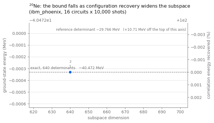
בניגוד לאינטואיציה, Backend רועש יותר יכול לתת חסם טוב מעט יותר מ-Backend נקי, מפני ששגיאות יוצרות חצאי-קונפיגורציות תקינים שהמעגל האידאלי לא היה דוגם לעולם, והרחבת תת-מרחב וריאציוני אינה יכולה להעלות את הערך העצמי הנמוך ביותר שלו. סימולציה רועשת יכולה להדגים את אותו אפקט; המדריך הזה מראה אותו עם דגימות חומרה.
# IBM Carbon palette: Blue 60 and Blue 80 for data, Gray 100/70/30 for ink and rules
SURFACE, INK, MUTED, RULE = "#ffffff", "#161616", "#6f6f6f", "#c6c6c6"
SERIES, DEEP, PURPLE = "#0f62fe", "#002d9c", "#6929c4"

def convergence_plot(
    history, e_ref, e_exact, title, colour=SERIES, full_dim=None
):
    """Energy against subspace dimension, scaled to the data rather than to the full window.

    A good run lands within a fraction of a percent of the exact answer, so an axis spanning
    reference-to-exact would squash every point onto one line.  The axis is therefore scaled to
    the data (plus the exact line, when there is one), and the right-hand axis carries the
    fraction of the correlation energy so the absolute and relative readings sit side by side.
    """
    dimensions = [h["dimension"] for h in history]
    energies = [h["energy"] for h in history]

    fig, ax = plt.subplots(figsize=(7.4, 4.3), facecolor=SURFACE)
    ax.set_facecolor(SURFACE)
    ax.plot(
        dimensions,
        energies,
        "-o",
        color=colour,
        linewidth=2,
        markersize=8,
        markeredgecolor=SURFACE,
        markeredgewidth=1.5,
        zorder=3,
    )
    stacked = {}
    for h in history:
        # a converged loop repeats the same point; stack the labels so they do not overprint
        key = (round(h["dimension"]), round(h["energy"], 9))
        offset = 12 + 11 * stacked.get(key, 0)
        stacked[key] = stacked.get(key, 0) + 1
        ax.annotate(
            str(h["iteration"]),
            xy=(h["dimension"], h["energy"]),
            xytext=(0, offset),
            textcoords="offset points",
            ha="center",
            fontsize=8,
            color=MUTED,
        )

    span = (max(dimensions) - min(dimensions)) or max(1, max(dimensions) // 4)
    x_left, x_right = (
        min(dimensions) - 0.14 * span,
        max(dimensions) + 0.40 * span,
    )
    ax.set_xlim(x_left, x_right)

    floor = min(energies) if e_exact is None else min(min(energies), e_exact)
    height = max(max(energies) - floor, 1e-3)
    ax.set_ylim(floor - 0.30 * height, max(energies) + 0.42 * height)

    if e_exact is not None:
        ax.axhline(
            e_exact, color=MUTED, linestyle="--", linewidth=1, zorder=1
        )
        label = "exact" + (f", {full_dim:,} determinants" if full_dim else "")
        ax.annotate(
            f"{label}   {e_exact:.3f} MeV".replace("-", "\u2212"),
            xy=(x_left, e_exact),
            xytext=(3, 5),
            textcoords="offset points",
            ha="left",
            va="bottom",
            color=MUTED,
            fontsize=9,
        )

    # the reference determinant is far off this scale; state it rather than plotting it
    ax.annotate(
        f"reference determinant {e_ref:.3f} MeV".replace("-", "\u2212")
        + f"   ({e_ref - max(energies):+.2f} MeV off the top of this axis)".replace(
            "-", "\u2212"
        ),
        xy=(x_right, max(energies) + 0.42 * height),
        xytext=(-3, -12),
        textcoords="offset points",
        ha="right",
        va="top",
        color=MUTED,
        fontsize=8.5,
    )

    if e_exact is not None and abs(e_exact - e_ref) > 1e-9:
        right = ax.twinx()
        low, high = ax.get_ylim()

        def to_percent(e):
            return 100 * (e - e_ref) / (e_exact - e_ref)

        right.set_ylim(to_percent(low), to_percent(high))
        right.set_ylabel("correlation energy recovered (%)", color=MUTED)
        right.tick_params(colors=MUTED)
        for side in ("top", "left"):
            right.spines[side].set_visible(False)
        right.spines["right"].set_color(MUTED)
        right.spines["bottom"].set_color(MUTED)

    ax.set_xlabel("subspace dimension", color=MUTED)
    ax.set_ylabel("ground-state energy (MeV)", color=MUTED)
    ax.set_title(title, color=INK, fontsize=11.5, loc="left", pad=12)
    ax.grid(axis="y", color=RULE, alpha=0.55)
    ax.tick_params(colors=MUTED)
    for side in ("top", "right"):
        ax.spines[side].set_visible(False)
    for side in ("bottom", "left"):
        ax.spines[side].set_color(MUTED)
    fig.tight_layout()
    return fig

convergence_plot(
    result_sd["history"],
    E_REF_SD,
    E_EXACT_SD,
    f"$^{{20}}$Ne: the bound falls as configuration recovery widens the subspace\n"
    f"({backend.name}, {N_CIRCUITS} circuits x {SHOTS:,} shots)",
    full_dim=len(basis_exact_sd),
)
plt.show()
דוגמת חומרה בקנה מידה גדול
הגדלת קנה המידה משנה רק את הקלטים, ולכן הצעד הבא הוא לשלב את ארבעת השלבים לפונקציה אחת ולהריץ אותה פעמיים, בשתי הפעמים על רגיסטר של 40 Qubits בקליפת מעל ליבת עם האינטראקציה GXPF1 [3].
שתי הריצות ממחישות היבטים שונים של הגדלת קנה המידה:
-
ל-, שני פרוטונים ולנטיים ושני נויטרונים ולנטיים, יש בסיס של 4,000 דטרמיננטות. הרגיסטר הוא 40 Qubits, אבל הבעיה עדיין קטנה מספיק כדי לאלכסן אותה במדויק על מחשב נייד, כך שאפשר להשוות את תוצאת החומרה להפניה מדויקת לאחר הגדלת גודל הרגיסטר.
-
ל-, ארבעה פרוטונים ולנטיים וארבעה נויטרונים ולנטיים, יש 1,963,461 דטרמיננטות מותרות לפי סימטריה באותם 40 Qubits. הפותר הצפוף של המדריך אינו יכול לאלכסן את כל המרחב הזה, ולכן הריצה מחזירה חסם עליון קפדני ואת דטרמיננטת הייחוס שהוא משפר.
עקבו אחר שני גדלים לאורך שתי הריצות. שיעור המאגר שנכנס בתוך תקציב השערים הקבוע מצטמצם ככל שהמאגר גדל, ו-pack_ensemble מדווח כמה נכלל. תת-המרחב מפסיק להיות מוגבל על ידי הדגימה ומתחיל להיות מוגבל על ידי MAX_DIMENSION, המטריצה הגדולה ביותר שהפותר הקלאסי הצפוף כאן בונה. בקנה מידה כזה, חישוב בייצור היה משתמש בפותר אינטראקציית קונפיגורציות נבחרת (selected-CI).
שילוב שלבים 1–4
הפונקציה הבאה קוראת לאותם שלבים כמו בהדרכה, באותו סדר.
def sqd_run(snt_file, n_protons, n_neutrons, name, exact=True):
    """The whole workflow for one nucleus.  Returns a record of every stage."""
    # -------------------------Step 1-------------------------
    ms = read_snt(DATA / snt_file, n_protons, n_neutrons)
    sp = m_scheme_states(ms)
    inter = Interaction(ms, sp)
    if sum(1 for s in sp if s.tz == -1) * 2 != len(sp):
        raise ValueError(
            f"{name}: post-selection needs equal proton and neutron state counts"
        )
    reference = reference_determinant(sp, inter, n_protons, n_neutrons)
    e_ref = matrix_element(inter, reference, reference)

    raw = excitation_pool(sp, reference)
    ranked = rank_pool(
        inter, reference, [op for op in raw if conserves_symmetry(sp, op)]
    )
    print(
        f"{name}: {len(sp)} qubits, {n_protons}p + {n_neutrons}n, A = {ms.mass_number}"
    )
    print(
        f"  2p2h pool {len(raw)} raw -> {len(ranked)} symmetry-allowed; "
        f"reference energy {e_ref:.6f} MeV"
    )

    # -------------------------Step 2-------------------------
    costs = excitation_costs(len(sp), ranked, costing_manager)
    circuits, bins, isa = pack_to_budget(
        len(sp),
        reference,
        ranked,
        costs,
        DEPTH_BUDGET,
        N_CIRCUITS,
        pass_manager,
    )
    packed = sum(len(b) for b in bins)
    worst = max(two_qubit_depth(c) for c in isa)
    worst_count = max(two_qubit_count(c) for c in isa)
    print(
        f"  packed {packed} of {len(ranked)} excitations; worst circuit two-qubit depth "
        f"{worst}, {worst_count} two-qubit gates"
    )

    # -------------------------Step 3-------------------------
    # a unique tag per run, so the jobs are findable later
    bit_arrays = sample(isa, SHOTS, JOB_TAGS + [name])
    matrix, probabilities, shots = pool_samples(bit_arrays, sp)
    survival = float(
        probabilities[
            (matrix[:, len(sp) // 2 :].sum(axis=1) == n_protons)
            & (matrix[:, : len(sp) // 2].sum(axis=1) == n_neutrons)
        ].sum()
    )
    print(
        f"  {shots:,} shots -> {len(matrix):,} distinct bitstrings, "
        f"{survival:.1%} of shots with the right nucleon numbers"
    )
    if survival == 0.0:
        raise RuntimeError(
            f"{name}: no shot carried the right nucleon numbers"
        )

    # -------------------------Step 4-------------------------
    result = recovery_loop(
        inter,
        sp,
        matrix,
        probabilities,
        reference,
        n_protons,
        n_neutrons,
        max_iterations=4,
        max_dimension=MAX_DIMENSION,
        seed=42,
    )
    energy = result["energy"]

    full_dim = count_basis(sp, n_protons, n_neutrons)  # cheap, even when huge
    e_exact = None
    if exact:
        full = full_basis(sp, n_protons, n_neutrons)
        if len(full) != full_dim:
            raise AssertionError(
                f"{name}: counted {full_dim} determinants but enumerated "
                f"{len(full)}"
            )
        e_exact, _ = ground_state(inter, full)

    print(f"  reference {e_ref:11.6f} MeV     pooled SQD {energy:11.6f} MeV")
    if e_exact is not None:
        print(
            f"  exact     {e_exact:11.6f} MeV  (dimension {full_dim})  ->  "
            f"{100 * (energy - e_ref) / (e_exact - e_ref):.1f}% of the correlation energy"
        )
        if energy < e_exact - 1e-7:
            raise AssertionError(
                f"{name}: pooled SQD bound is below the exact energy"
            )
    else:
        print(
            f"  no exact reference: the symmetry-allowed basis is {full_dim:,} determinants"
        )
        print(
            f"  the bound captures {energy - e_ref:.6f} MeV of correlation energy"
        )
    print()

    return dict(
        name=name,
        qubits=len(sp),
        pool=len(ranked),
        packed=packed,
        two_qubit=worst,
        two_qubit_gates=worst_count,
        shots=shots,
        distinct=len(matrix),
        survival=survival,
        dimension=len(result["basis"]),
        full_dim=full_dim,
        e_ref=e_ref,
        e_sqd=energy,
        e_exact=e_exact,
        history=result["history"],
        # the subspace and its eigenvector cannot be reconstructed from the summary --
        # they depend on the sampled shots -- so keep them for the scaling analysis
        interaction=inter,
        states=sp,
        reference=reference,
        ranked=ranked,
        basis=result["basis"],
        vector=result["vector"],
    )

pretty = {"20Ne": "$^{20}$Ne", "44Ti": "$^{44}$Ti", "48Cr": "$^{48}$Cr"}

small_scale = dict(
    name="20Ne",
    qubits=len(sp_sd),
    pool=len(ranked_sd),
    packed=PACKED_SD,
    two_qubit=worst_sd,
    two_qubit_gates=worst_count_sd,
    shots=shots_sd,
    distinct=len(matrix_sd),
    survival=shot_survival_sd,
    dimension=len(result_sd["basis"]),
    full_dim=len(basis_exact_sd),
    e_ref=E_REF_SD,
    e_sqd=E_SQD_SD,
    e_exact=E_EXACT_SD,
    history=result_sd["history"],
    interaction=inter_sd,
    states=sp_sd,
    reference=occ_sd,
    ranked=ranked_sd,
    basis=result_sd["basis"],
    vector=result_sd["vector"],
)
: אותה זרימת עבודה על רגיסטר של 40 Qubits
לקליפת מעל יש ארבעה אורביטלים לכל סוג חלקיק ו-20 תתי-מצבים מגנטיים בכל אחד, ולכן הרגיסטר הוא 40 Qubits. שני פרוטונים ולנטיים ושני נויטרונים ולנטיים יוצרים את , עם 4,000 דטרמיננטות מותרות לפי סימטריה — כפי שש מונים מבסיס , תוך שימוש ב-40 Qubits במקום 24.
זו הגדולה מבין שתי הדוגמאות ש-Notebook יכול לפתור במדויק, כך שאפשר להשוות את תוצאת החומרה להפניה מדויקת.
large_scale_verified = sqd_run("gxpf1.snt", 2, 2, "44Ti", exact=True)
44Ti: 40 qubits, 2p + 2n, A = 44
  2p2h pool 1602 raw -> 174 symmetry-allowed; reference energy -44.309387 MeV
  packed 96 of 174 excitations; worst circuit two-qubit depth 272, 285 two-qubit gates
job dap31a02fm4c73f67dp0: 16 circuits x 10,000 shots on ibm_phoenix
  160,000 shots -> 48,170 distinct bitstrings, 18.6% of shots with the right nucleon numbers
  iteration 1: 187 proton x 189 neutron halves -> dimension 3891, E = -47.849086 MeV
  iteration 2: 190 proton x 190 neutron halves -> dimension 4000, E = -47.876666 MeV
  iteration 3: 190 proton x 190 neutron halves -> dimension 4000, E = -47.876666 MeV
  reference  -44.309387 MeV     pooled SQD  -47.876666 MeV
  exact      -47.876666 MeV  (dimension 4000)  ->  100.0% of the correlation energy
: מעבר ליכולת האלכסון המדויק של המדריך
הוספת שני פרוטונים ושני נויטרונים משתמשת באותו רגיסטר של 40 Qubits (4, 4 עבור ) ומגדילה את גודל הבסיס בגורם של כ-491, ל-1,963,461 דטרמיננטות מותרות לפי סימטריה. המטריצה הזו רחוקה בהרבה ממה שהמדריך הזה יבנה, ולכן exact=False: אין אנרגיית ייחוס מדויקת, רק החסם הוריאציוני ודטרמיננטת הייחוס שהוא משפר.
שני דברים משתנים בקנה מידה הזה, ושניהם נראים בפלט. המאגר גדל למאות עירורים מותרים, ולכן תקציב השערים הקבוע מכסה עכשיו רק חלק קטן ממנו ולא את כולו. בנוסף, תת-המרחב המכפלתי שהדגימות פורשות גדול מ-MAX_DIMENSION, ולכן הפותר הצפוף קוצץ אותו לפי משקל הדגימה. החסם נשאר קפדני, אבל הוא עשוי להיות פחות מדויק מחסם שמחושב מכל התצורות שנדגמו. חישוב ייצורי היה שומר את הדגימות ומשתמש בפותר שתומך בתת-מרחב גדול יותר.
large_scale_unverified = sqd_run("gxpf1.snt", 4, 4, "48Cr", exact=False)
48Cr: 40 qubits, 4p + 4n, A = 48
  2p2h pool 5536 raw -> 582 symmetry-allowed; reference energy -93.041237 MeV
  packed 96 of 582 excitations; worst circuit two-qubit depth 224, 279 two-qubit gates
job dap32a02fm4c73f67eog: 16 circuits x 10,000 shots on ibm_phoenix
  160,000 shots -> 55,436 distinct bitstrings, 18.6% of shots with the right nucleon numbers
  iteration 1: 223 proton x 223 neutron halves -> dimension 3977, E = -96.481598 MeV
  iteration 2: 223 proton x 223 neutron halves -> dimension 3977, E = -96.481598 MeV
  reference  -93.041237 MeV     pooled SQD  -96.481598 MeV
  no exact reference: the symmetry-allowed basis is 1,963,461 determinants
  the bound captures -3.440361 MeV of correlation energy
הערכת תוצאה בלי ייחוס מדויק
להרצת אין ייחוס מדויק במסגרת המדריך הזה. השתמשו בדגימות הקיימות כדי להעריך התכנסות ולהשוות לקו הבסיס של הבחירה הקלאסית, בלי זמן QPU נוסף ובלי אלכסון של המרחב המלא.
האם זה התכנס? סדרו מחדש את הדטרמיננטות שנשמרו לפי המשקל שלהן בווקטור העצמי המתכנס, ותת-המרחבים נעשים מקוננים. אז אלכסון של הבלוק המוביל בגודל עבור סולם של ערכי מתאר את ירידת החסם על פני שני סדרי גודל של גודל תת-המרחב. אם החסם עדיין יורד בחדות ב- הגדול ביותר, מגבלת המימד של הפותר הקלאסי היא האילוץ הקובע, ו-MAX_DIMENSION הוא הפרמטר שכדאי להגדיל. אם הוא התייצב, הוספת עוד דטרמיננטות שנשמרו תשפר מעט; התקדמות נוספת עשויה לדרוש דגימה של תצורות נוספות. ההמילטוניאן נבנה פעם אחת בגודל מלא וכל שלב הוא בלוק ראשי שלו, ולכן הסריקה כולה עולה בניית מטריצה אחת ולא אחת לכל שלב.
איך דגימה קוונטית משתווה לבחירה קלאסית? השוו מול תת-מרחב באותו גודל שנבחר בהליך הבחירה הקלאסי: קחו את המאגר מדורג לפי תורת הפרעות בסדר הציונים, הגדילו את תת-המרחב המכפלתי לאותו מימד ואלכסנו אותו במקום. שתי העקומות הן חסמים עליונים קפדניים לאותו המילטוניאן, ולכן זו שנמצאת נמוך יותר באותו מימד בחרה דטרמיננטות טובות יותר. ההשוואה הזו קובעת אם דגימה בחומרה משפרת את הערכת האנרגיה ביחס לקו הבסיס הקלאסי.
תת-המרחב הזה לא נבחר עבור מצבים מעוררים. שחזור תצורות מכוון את תת-המרחב לפי תפוסות מצב היסוד, ולכן הערכים העצמיים הגבוהים רחוקים הרבה יותר מהתכנסות מהנמוך ביותר, ואנרגיית העירור הראשונה יוצאת גבוהה בהרבה מה- שנמדד. כדי להגיע למצבים מעוררים כראוי צריך תת-מרחב שנבחר עבורם.
def subspace_scaling(
    inter, basis, vector, points=18, smallest=32, largest=None
):
    """Nested Rayleigh-Ritz sweep: the lowest eigenvalue of the leading d x d block, for a ladder of d.

    Reordering the basis by descending weight in the converged eigenvector makes every subspace in
    the ladder a subset of the next, so the energies fall monotonically and each one is a valid
    variational bound.  H is built once at full size; each rung is a principal block.
    """
    order = np.argsort(-(np.abs(vector) ** 2))
    ordered = [basis[i] for i in order]
    weights = (np.abs(vector) ** 2)[order]
    if (
        largest is not None
    ):  # cap the ladder so two subspaces end at a common dimension
        ordered, weights = ordered[:largest], weights[:largest]
    H = subspace_hamiltonian(inter, ordered)
    dimensions = np.unique(
        np.geomspace(smallest, len(ordered), points).astype(int)
    )
    rows = [
        (
            int(d),
            float(
                eigh(H[:d, :d], eigvals_only=True, subset_by_index=[0, 0])[0]
            ),
        )
        for d in dimensions
    ]
    return rows, np.cumsum(weights)

def classical_selection(
    inter, sp, reference, ranked, target, n_protons, n_neutrons
):
    """The subspace classical perturbative ranking would pick, grown to `target` dimension.

    Same product construction as the sampled subspace, and the same truncation discipline -- half
    configurations are offered to `grow_subspace` in order of importance and it takes as many as
    fit.  The only difference from the sampled path is where the ordering comes from: PT2 score
    here, measured sampling weight there.  So the comparison isolates *which determinants got
    chosen* and nothing else.

    Truncating by any other rule would not be a fair baseline.  Slicing an arbitrarily ordered
    list, for instance, keeps determinants by accident rather than by importance and makes the
    classical subspace look worse than classical selection really is.
    """
    p_ref = tuple(i for i in reference if sp[i].tz == -1)
    n_ref = tuple(i for i in reference if sp[i].tz == +1)
    reached = {reference}
    proton_order, neutron_order = [p_ref], [n_ref]
    seen_p, seen_n = {p_ref}, {n_ref}
    product_budget = 4 * target

    for op, _, _ in ranked:  # ranked is already in descending PT2 score
        h1, h2, v1, v2 = op
        fresh = {
            tuple(sorted(set(d) - {h1, h2} | {v1, v2}))
            for d in reached
            if {h1, h2} <= set(d) and not {v1, v2} & set(d)
        }
        reached |= fresh
        for det in fresh:  # first appearance fixes a half's rank
            half_p = tuple(i for i in det if sp[i].tz == -1)
            half_n = tuple(i for i in det if sp[i].tz == +1)
            if half_p not in seen_p:
                seen_p.add(half_p)
                proton_order.append(half_p)
            if half_n not in seen_n:
                seen_n.add(half_n)
                neutron_order.append(half_n)
        if len(proton_order) * len(neutron_order) > product_budget:
            # Half-configuration products over-count the subspace, because only the
            # symmetry-allowed ones survive `product_subspace`.  Stopping on the product
            # count alone can therefore leave the basis far short of `target`, so check
            # the dimension actually realized and widen the budget if it falls short.
            trial, _, _ = grow_subspace(
                sp,
                [p_ref],
                [n_ref],
                proton_order,
                neutron_order,
                n_protons,
                n_neutrons,
                max_dimension=target,
            )
            if len(trial) >= target:
                break
            product_budget *= 2

    basis, _, _ = grow_subspace(
        sp,
        [p_ref],
        [n_ref],
        proton_order,
        neutron_order,
        n_protons,
        n_neutrons,
        max_dimension=target,
    )
    return basis

run = large_scale_unverified
if "basis" not in run:
    raise RuntimeError(
        "this cell needs the subspace and eigenvector that sqd_run now returns; "
        "re-run the sqd_run definition and the 48Cr cell"
    )

print(
    f"{run['name']}: sweeping nested subspaces of the sampled basis "
    f"(dimension {run['dimension']})"
)
sampled_rows, cumulative = subspace_scaling(
    run["interaction"], run["basis"], run["vector"]
)

print(
    f"{run['name']}: building the classically selected subspace at the same dimension"
)
classical_basis = classical_selection(
    run["interaction"],
    run["states"],
    run["reference"],
    run["ranked"],
    run["dimension"],
    4,
    4,
)
# Both subspaces must be scored at the same dimension.  Symmetry filtering can still leave
# the classical construction short of the target when the ranked pool runs out, so take the
# dimension both actually reach, cap both ladders there, and verify they agree.
common_dim = min(sampled_rows[-1][0], len(classical_basis))
if common_dim < sampled_rows[-1][0]:
    sampled_rows, _ = subspace_scaling(
        run["interaction"], run["basis"], run["vector"], largest=common_dim
    )
classical_rows, _ = subspace_scaling(
    run["interaction"],
    classical_basis,
    ground_state(run["interaction"], classical_basis)[1],
    largest=common_dim,
)
if sampled_rows[-1][0] != classical_rows[-1][0]:
    raise RuntimeError(
        f"comparison dimensions differ: sampled {sampled_rows[-1][0]}, "
        f"classical {classical_rows[-1][0]}"
    )

advantage = sampled_rows[-1][1] - classical_rows[-1][1]
direction = "lower" if advantage < 0 else "higher"
verdict = "beats" if advantage < 0 else "does not beat"
descent = next(
    e for d, e in reversed(sampled_rows) if d <= sampled_rows[-1][0] / 2
)
for fraction in (0.90, 0.99):
    count = int(np.searchsorted(cumulative, fraction) + 1)
    print(
        f"  {fraction:.0%} of the eigenvector norm sits on {count} determinants "
        f"({count / run['full_dim']:.1e} of the {run['full_dim']:,}-determinant space)"
    )
print(
    f"  bound still falling {1000 * (sampled_rows[-1][1] - descent):+.1f} keV "
    f"over the last doubling of dimension"
)
print(
    f"  sampled {sampled_rows[-1][1]:.6f} MeV vs classically selected "
    f"{classical_rows[-1][1]:.6f} MeV at a verified common dimension of "
    f"{classical_rows[-1][0]:,}"
)
print(
    f"  -> the sampled subspace is {abs(advantage) * 1000:.0f} keV {direction}"
)
48Cr: sweeping nested subspaces of the sampled basis (dimension 3977)
48Cr: building the classically selected subspace at the same dimension
  90% of the eigenvector norm sits on 107 determinants (5.4e-05 of the 1,963,461-determinant space)
  99% of the eigenvector norm sits on 593 determinants (3.0e-04 of the 1,963,461-determinant space)
  bound still falling -15.6 keV over the last doubling of dimension
  sampled -96.481598 MeV vs classically selected -95.314510 MeV at a verified common dimension of 3,957
  -> the sampled subspace is 1167 keV lower
fig, axes = plt.subplots(1, 2, figsize=(11.2, 4.0), facecolor=SURFACE)

# left: two nested convergence curves on the same axes
ax = axes[0]
ax.set_facecolor(SURFACE)
ax.plot(
    [d for d, _ in sampled_rows],
    [e for _, e in sampled_rows],
    "-o",
    color=SERIES,
    linewidth=2,
    markersize=5,
    markeredgecolor=SURFACE,
    markeredgewidth=1,
    zorder=4,
    label="sampled on the QPU",
)
ax.plot(
    [d for d, _ in classical_rows],
    [e for _, e in classical_rows],
    "--s",
    color=MUTED,
    linewidth=1.6,
    markersize=4,
    markeredgecolor=SURFACE,
    markeredgewidth=1,
    zorder=3,
    label="classically selected, same size",
)
ax.axhline(run["e_ref"], color=RULE, linestyle=":", linewidth=1.2, zorder=1)
ax.annotate(
    f"reference determinant {run['e_ref']:.2f} MeV".replace("-", "\u2212"),
    xy=(sampled_rows[-1][0], run["e_ref"]),
    xytext=(-2, 4),
    textcoords="offset points",
    ha="right",
    va="bottom",
    color=MUTED,
    fontsize=8,
)

# mark the gap between the two curves at the largest dimension, not either curve alone
edge = sampled_rows[-1][0]
ax.plot(
    [edge, edge],
    [classical_rows[-1][1], sampled_rows[-1][1]],
    "-",
    color=SERIES,
    linewidth=1.0,
    alpha=0.7,
    zorder=2,
)
ax.annotate(
    f"{abs(advantage) * 1000:.0f} keV {direction}\nat equal dimension",
    xy=(edge, 0.5 * (classical_rows[-1][1] + sampled_rows[-1][1])),
    xytext=(-8, 0),
    textcoords="offset points",
    ha="right",
    va="center",
    color=SERIES,
    fontsize=8.5,
)

ax.set_xscale("log")
ax.set_xlim(sampled_rows[0][0] * 0.75, edge * 1.5)
ax.set_xlabel("subspace dimension", color=MUTED)
ax.set_ylabel("variational upper bound (MeV)", color=MUTED)
ax.set_title(
    f"{pretty[run['name']]}: the bound, and the subspace it {verdict}",
    color=INK,
    fontsize=11,
    loc="left",
    pad=10,
)
legend = ax.legend(frameon=False, fontsize=8.5, loc="lower left")
for text in legend.get_texts():
    text.set_color(MUTED)

# right: why a few thousand determinants can bound two million
ax = axes[1]
ax.set_facecolor(SURFACE)
ranks = np.arange(1, len(cumulative) + 1)
ax.plot(ranks, 100 * cumulative, "-", color=DEEP, linewidth=2, zorder=3)
for fraction, style, label_y in ((0.90, ":", 46), (0.99, "--", 24)):
    count = int(np.searchsorted(cumulative, fraction) + 1)
    ax.axvline(count, color=MUTED, linestyle=style, linewidth=1, zorder=1)
    ax.annotate(
        f"{fraction:.0%} of the norm\non {count} determinants",
        xy=(count, label_y),
        xytext=(7, 0),
        textcoords="offset points",
        ha="left",
        va="center",
        color=MUTED,
        fontsize=8.5,
    )
ax.set_xscale("log")
ax.set_xlim(0.8, len(cumulative) * 2.6)
ax.set_ylim(0, 104)
ax.set_xlabel("determinants, ordered by weight", color=MUTED)
ax.set_ylabel("cumulative share of the eigenvector (%)", color=MUTED)
ax.set_title(
    f"Sparsity: {run['full_dim']:,} determinants in the sector",
    color=INK,
    fontsize=11,
    loc="left",
    pad=10,
)

for ax in axes:
    ax.grid(axis="y", color=RULE, alpha=0.55)
    ax.tick_params(colors=MUTED, labelsize=8.5)
    for side in ("top", "right"):
        ax.spines[side].set_visible(False)
    for side in ("bottom", "left"):
        ax.spines[side].set_color(MUTED)
fig.tight_layout()
plt.show()
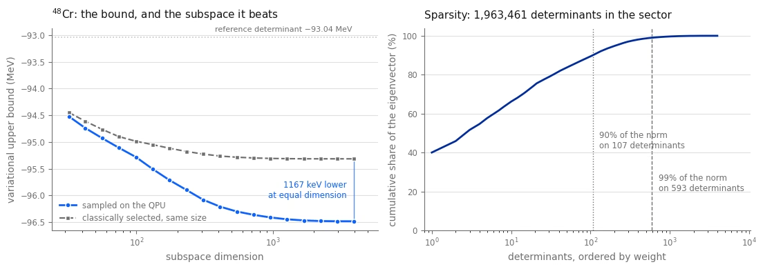
השוואת שלוש ההרצות
אי אפשר להשוות אנרגיות מוחלטות בין גרעינים שונים ואינטראקציות שונות, ולכן התמקדו בחלק מאנרגיית המתאם שהושב בין ההרצות, במקום שבו יש ייחוס מדויק. השוו גם את עומק המעגל ואת חלק הדגימות (shots) שנזרקו.
runs = [small_scale, large_scale_verified, large_scale_unverified]

print(
    f"{'run':>6}  {'qubits':>6}  {'pool':>9}  {'2q depth':>8}  {'2q gates':>8}  "
    f"{'shots kept':>10}  {'dim':>6}  {'of':>9}  {'% corr':>7}"
)
for r in runs:
    fraction = (
        "--"
        if r["e_exact"] is None
        else f"{100 * (r['e_sqd'] - r['e_ref']) / (r['e_exact'] - r['e_ref']):.1f}%"
    )
    coverage = "{}/{}".format(r["packed"], r["pool"])
    print(
        f"{r['name']:>6}  {r['qubits']:>6}  {coverage:>9}  "
        f"{r['two_qubit']:>8}  {r['two_qubit_gates']:>8}  {r['survival']:>9.1%}  "
        f"{r['dimension']:>6}  {(r['full_dim'] or 0):>9,}  {fraction:>7}"
    )

print()
for r in runs:
    exact = (
        f"exact {r['e_exact']:11.6f}"
        if r["e_exact"] is not None
        else "exact  unavailable"
    )
    print(
        f"{r['name']:>6}   reference {r['e_ref']:11.6f}   pooled SQD {r['e_sqd']:11.6f}   {exact} MeV"
    )
run  qubits       pool  2q depth  2q gates  shots kept     dim         of   % corr
  20Ne      24      78/78       228       234      31.5%     640        640   100.0%
  44Ti      40     96/174       272       285      18.6%    4000      4,000   100.0%
  48Cr      40     96/582       224       279      18.6%    3977  1,963,461       --

  20Ne   reference  -29.765549   pooled SQD  -40.472331   exact  -40.472331 MeV
  44Ti   reference  -44.309387   pooled SQD  -47.876666   exact  -47.876666 MeV
  48Cr   reference  -93.041237   pooled SQD  -96.481598   exact  unavailable MeV
# Left: how much of the correlation energy was recovered, where the exact answer is known.
# Right: the bound itself for the run that has nothing to score against.
scored = [r for r in runs if r["e_exact"] is not None]

fig, ax = plt.subplots(figsize=(6.4, 3.9), facecolor=SURFACE)
ax.set_facecolor(SURFACE)
labels = [
    f"{pretty[r['name']]}\n{r['qubits']} qubits\n{r['full_dim']:,} determinants"
    for r in scored
]
fractions = [
    100 * (r["e_sqd"] - r["e_ref"]) / (r["e_exact"] - r["e_ref"])
    for r in scored
]
shades = [SERIES, DEEP, PURPLE]
bars = ax.bar(
    labels, fractions, width=0.46, color=shades[: len(scored)], zorder=3
)
for bar, fraction, r in zip(bars, fractions, scored):
    ax.annotate(
        f"{fraction:.1f}%",
        xy=(bar.get_x() + bar.get_width() / 2, fraction),
        xytext=(0, 5),
        textcoords="offset points",
        ha="center",
        va="bottom",
        color=INK,
        fontsize=10,
    )
    ax.annotate(
        f"dim {r['dimension']:,}",
        xy=(bar.get_x() + bar.get_width() / 2, 3),
        ha="center",
        va="bottom",
        color=SURFACE,
        fontsize=8.5,
    )
ax.axhline(100, color=MUTED, linestyle="--", linewidth=1, zorder=1)
ax.annotate(
    "exact diagonalization",
    xy=(-0.45, 100),
    xytext=(0, 4),
    textcoords="offset points",
    ha="left",
    va="bottom",
    color=MUTED,
    fontsize=8.5,
)
ax.set_ylim(0, 118)
ax.set_ylabel("correlation energy recovered (%)", color=MUTED)
ax.set_title(
    f"Where the exact answer is known ({backend.name})",
    color=INK,
    fontsize=11,
    loc="left",
    pad=10,
)
ax.grid(axis="y", color=RULE, alpha=0.55)
ax.tick_params(colors=MUTED, labelsize=8.5)
for side in ("top", "right"):
    ax.spines[side].set_visible(False)
for side in ("bottom", "left"):
    ax.spines[side].set_color(MUTED)
fig.tight_layout()
plt.show()

# the same convergence view as the walkthrough, for the run with no exact reference
convergence_plot(
    large_scale_unverified["history"],
    large_scale_unverified["e_ref"],
    None,
    f"{pretty[large_scale_unverified['name']]}: "
    f"{large_scale_unverified['full_dim']:,} determinants, no exact answer to score against\n"
    f"({backend.name}, {N_CIRCUITS} circuits x {SHOTS:,} shots)",
    colour=DEEP,
)
plt.show()

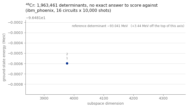
סיכום
זרימת עבודה אחת, ללא שינוי מלבד הקלטים שלה, רצה על QPU בשלושה גדלי בעיה: בעיה של 24 קיוביטים שאפשר לבדוק במדויק, בעיה של 40 קיוביטים שעדיין אפשר לבדוק במדויק, ובעיה של 40 קיוביטים עם כמעט שני מיליון מצבי בסיס, מעבר ליכולת האלכסון המדויק של המדריך הזה.
שלוש ההרצות ממחישות את הנקודות הבאות:
-
השלב הקוונטי רק צריך להציע דטרמיננטות. המעגל קבוע, מוזן מתורת הפרעות מסדר שני ולעולם לא עובר אופטימיזציה. שום דבר בזרימת העבודה לא דורש שהאמפליטודות שלו יהיו מדויקות, רק שהתומך שלו יהיה שימושי. אלכסון קלאסי בתת-המרחב שנבחר נותן חסם עליון וריאציוני, אם כי החסם משתנה עם התצורות שנדגמו.
-
עירורי קיוביטים מקטינים את עומק המעגל. מכיוון שרק התומך חשוב, אפשר להחליף את בלוקי העירור הפרמיוניים בעירורי קיוביטים, שעלותם לא גדלה עם המרחק בין האורביטלים שהם מחברים. שלב 2 מדד את החיסכון ב-Backend בפועל, וזה ההבדל בין מעגל שנכנס בנוחות בתוך זמן הקוהרנטיות לבין מעגל שלא.
-
שחזור תצורות ממחזר דגימות רועשות. כל shot עם מספר פרוטונים או נייטרונים שגוי מתוקן לפי הערכת התפוסה הנוכחית ולא נזרק, וכל חצי-תצורה מתוקנת יכולה להוסיף תצורות לתת-המרחב. הרחבת תת-מרחב וריאציוני לא יכולה להעלות את הערך העצמי הנמוך ביותר שלו. המדריך הזה מדגים שחזור תצורות באמצעות דגימות מהחומרה.
-
האילוץ הקובע משתנה עם הגדלת הקנה מידה. ב-24 קיוביטים ה-ansatz יכול היה להגיע לתשובה המדויקת, ורק הדגימה עמדה בדרך. ב-40 קיוביטים עם ארבעה נוקלאונים ואלנטיים לכל סוג, תקציב השערים מכסה רק חלק קטן מהמאגר והפותר הקלאסי הצפוף מגביל את תת-המרחב. לדעת איזה משלושת הגורמים מגביל אתכם היא המיומנות המעשית שזרימת העבודה הזו מלמדת.
השלבים הבאים
עיינו במשאבים הקשורים האלה:
-
דיאגונליזציה קוונטית מבוססת דגימות של המילטוניאן כימי: אותו אלגוריתם מיושם על מבנה אלקטרוני, באמצעות פותר ה-selected-CI של תוסף SQD.
-
תיעוד תוסף SQD: כלי עזר לבחירה לאחר מעשה, לדגימת משנה ולשחזור תצורות.
-
אלגוריתמי דיאגונליזציה קוונטית: קורס מלא על דיאגונליזציה של תת-מרחבים, כולל גרסאות Krylov.
-
מבוא לטרנספילציה: אפשרויות מנהל המעברים החשובות כשהמעגל נשלט על ידי שערי שני קיוביטים.
-
מצבי הרצה: גלו את batch mode לתזמון משימות בלתי תלויות.
הרחבות שכדאי לשקול
-
החליפו את הפותר הצפוף.
MAX_DIMENSIONהוא התקרה לכל דבר בקנה המידה של , ו-np.linalg.eighעל מטריצה צפופה הוא הסיבה לכך. בניית אותו ההמילטוניאן המוטל כמטריצה דלילה ושימוש בפותר עצמי איטרטיבי כמוscipy.sparse.linalg.eigsh, או בפותר Davidson או selected-CI שתוכנן לאינטראקציות גרעיניות דו-גופיות, יכולים לתמוך בתת-מרחבים גדולים יותר. הגבול המעשי תלוי בדלילות המטריצה, בזיכרון הזמין ובהתכנסות הפותר, והמדריך הזה לא בוחן הרחבה זו. הפונקציהqiskit_addon_sqd.fermion.solve_sciשל תוסף SQD אינה תחליף ישיר: היא עוטפת פותר למבנה אלקטרוני וצפויה לקבל אינטגרלים חד-גופיים ודו-גופיים בצורה הזו, ולכן מבנה המכפלה המשותף פרוטון נייטרון אינו מספיק בפני עצמו. שימוש בה ידרוש מיפוי של אינטראקציית מודל הקליפות ממשוואה (1) לאינטגרלים האלה ואימות התוצאה מול האנרגיות המדויקות שהמחברת הזו כבר מחשבת. -
הוסיפו batching ודגימת משנה. זרימת העבודה המפורסמת של pooled SQD מאלכסנת כמה דגימות משנה בלתי תלויות בכל איטרציה ושומרת את הטובה ביותר. המדריך הזה משתמש באצווה אחת בכל איטרציה, מה שלא מזיק לחסם הווריאציוני אך אינו מספק את מידע השונות שמעיד אם עוד shots היו עוזרים.
-
מצבים מעוררים ומגזרים אחרים. הערכים העצמיים הגבוהים של כל המילטוניאן תת-מרחב הם חסמים עליונים למצבים מעוררים באותו גזרת סימטריה, והרצה ב- מגיעה לגזרות אחרות. בדיקת ה- בשלב 1 היא כבר חצי מהחישוב הזה.
-
מרחב מודל חוצה-קליפות. הזוגיות מתקיימת אוטומטית בתוך קליפה עיקרית אחת, ולכן היא לא עושה כאן עבודה. מרחב - מערבב זוגיויות של ומשנה את הזוגיות לאילוץ רביעי אמיתי, כזה שלא תיתפס לבדה לא על ידי התיקון של SQD לפי משקל המינג ולא על ידי בניית המכפלה.
-
גרעינים בעלי מסה אי-זוגית.
reference_determinantדורש מספר ואלנטי זוגי בכל סוג, משום שמילוי זוגי הפוך-זמן הוא מה שכופה . גרעין אי-זוגי דורש יעד חצי-שלם והתייחסות לא מזווגת.
נספח
הסעיף הזה מסביר את ההיגיון שמאחורי פונקציות העזר שהוצגו בסעיף ההגדרה.
למה אי אפשר לוותר על שינוי קנה המידה לפי תלות במסה
אינטראקציות אמפיריות של מודל הקליפות מותאמות במסה אחת ומיושמות על שרשרת איזוטופים, כשאברי המטריצה הדו-גופיים מוכפלים ב-. בשני קובצי האינטראקציה , עם למשפחת USD ו- ל-GXPF1. בשורת הכותרת הדו-גופית של קובץ .snt, שני המספרים האלה יושבים במקום שבו סביר למצוא תדר אוסילטור ואנרגיית ליבה, ולכן קל לפרש אותם לא נכון; קריאת המעריך כאנרגיית ליבה קבועה מוסיפה היסט מלאכותי לכל איבר אלכסוני ומשמיטה את שינוי קנה המידה, ומשנה את אנרגיית המתאם בכמה אחוזים. בדיקת הסימטריה בשלב 1 לא מאמתת בפני עצמה את סולם האנרגיה. השוואת אנרגיית העירור של , הנמדדת ב-MeV, לניסוי מספקת בדיקה נוספת של שינוי קנה המידה התלוי במסה. אנרגיית עירור היא הפרש בין רמות, ולכן היא לא מגלה היסט קבוע שהוחל על כל האנרגיות.
למה הייחוס נמצא בחיפוש ולא במילוי
הייחוס המובן מאליו הוא הדטרמיננטה שממלאת את האנרגיות הנמוכות ביותר של חלקיק יחיד. היא אינה הדטרמיננטה בעלת האנרגיה הנמוכה ביותר, כי האלכסון של משוואה (1) כולל את האיבר הדו-גופי , ואינטראקציית הזיווג מעדיפה בחוזקה לאכלס שותפים הפוכי-זמן ב- הגדול ביותר שזמין. בקליפת זה ההבדל בין הזוג לזוג של , והוא שווה בערך 1 MeV; בקליפת הוא שווה קרוב ל-2. מכיוון שאנרגיית הייחוס מגדירה את האפס של מדד "אנרגיית המתאם שהושבה", בחירה גרועה מנפחת את המדד ונותנת נקודת התחלה פחות מדויקת.
הגבלה למילויים זוגיים הופכת חיפוש ממצה לזול, עם מועמדים לכל סוג (לכל היותר כמה אלפים), ומבטיחה . בכל מקרה במדריך הזה שאפשר לבדוק מול ספירה מלאה, החיפוש מחזיר את הדטרמיננטה בעלת האלכסון הנמוך ביותר ברמה הגלובלית, שהיא גם המרכיב היחיד הגדול ביותר של מצב היסוד המדויק.
למה האמפליטודה מסדר ראשון ולא הזווית המדויקת של שתי רמות
אלכסון ההמילטוניאן במרחב נותן את זווית הערבוב ; אפשר להתפתות לקרוא לה הבחירה הנכונה עבור זוג רמות מבודד. ב-ansatz הזה כמה עשרות בלוקי עירור פועלים ברצף על אותו ייחוס, ולכן אופטימיזציה של כל בלוק בנפרד לא בהכרח מייעלת את המעגל המורכב.
תפקיד המעגל קובע את בחירת הזווית. מכיוון ש- לכל ממשי, הזווית המדויקת תמיד קטנה בגודלה מהאמפליטודה מסדר ראשון , ולכן תמיד משאירה יותר אמפליטודה על דטרמיננטת הייחוס. מעגל ששומר יותר אמפליטודה על הייחוס מחזיר את הייחוס לעתים קרובות יותר ודטרמיננטות מעוררות שונות לעתים רחוקות יותר. ב-pooled SQD, הפלט השימושי של shot הוא דטרמיננטה שהשלב הקלאסי עוד לא ראה, וזה מה שמניע שימוש בזווית הגדולה יותר במדריך הזה. אף אחת מהזוויות לא צריכה להיות מדויקת, כי האלכסון הקלאסי משליך את האמפליטודות של המעגל לגמרי ומפיק אמפליטודות משלו.
למה pooled SQD יכול להשתמש בעירורי קיוביטים
העירור הפרמיוני ממופה תחת Jordan-Wigner לשמונה מחרוזות פאולי, שכל אחת נושאת אופרטורי על כל קיוביט שבין האינדקסים החיצוניים ביותר. המחרוזות האלה מקודדות את הסימן הפרמיוני, ועלותן גדלה עם המרחק, שבעירור פרוטון-נייטרון הוא כל האוגר.
מחיקתן נותנת את אופרטור עירור הקיוביטים של Yordanov ואחרים [5]. זה אופרטור שונה: המצב שהוא מכין שונה מהפרמיוני בסימנים של האמפליטודות שלו, ושתי התפלגויות הדגימה יכולות להיות שונות מאוד. מה שהוא לא משנה הוא אילו דטרמיננטות בעלות אמפליטודה שונה מאפס, כי כל בלוק עדיין מסובב בתוך אותו מרחב דו-ממדי לכל דטרמיננטה שעליה הוא פועל, ועדיין משמר במדויק את שני מספרי הנוקלאונים, את ואת הזוגיות. לכן קבוצת הדטרמיננטות הנגישה זהה, והיא הדבר היחיד ש-pooled SQD משתמש בו; האלכסון הקלאסי מקצה אמפליטודות משלו בכל מקרה. שלב 2 מאמת את טענת התומך הזהה על אופרטור אמיתי מהמאגר ומודד כמה ההחלפה חוסכת.
המגבלה היא שהמשקלים של הדגימה שונים, ולכן שתי הבניות לא יגלו דטרמיננטות באותו סדר בכמות shots סופית. מכיוון שהדירוג שמחליט אילו עירורים נכנסים למעגלים הוא קלאסי ולא משתנה, והשלב הקלאסי ממילא משקלל הכול מחדש, ההבדל במשקלי הדגימה הוא פשרה תמורת עומק מעגל מופחת.
למה שייך לשלב המכפלה
בחירה לאחר מעשה ושחזור תצורות פועלים שניהם על משקלי המינג: מספר הפרוטונים בחצי אחד של האוגר ומספר הנייטרונים בחצי השני. אינו מהצורה הזו. זו תכונה של תצורת פרוטונים המזווגת עם תצורת נייטרונים. shot שחצי הפרוטונים וחצי הנייטרונים שלו נושאים כל אחד את מספר הנוקלאונים הנכון מכיל שתי חצאי-תצורות שימושיות גם כשערכי ה- שלהן לא מתקזזים, כי חצי הפרוטונים ב- מצוין ברגע שהוא מזווג עם חצי נייטרונים ב-. סינון shots שלמים לפי הכולל זורק את שני החצאים, והטלת על המכפלות המשולבות מחדש שומרת אותם. אותו טיעון מסביר למה recover_configurations לא צריכה שום מושג של כדי להועיל במקרה הזה.
מקורות
-
J. Robledo-Moreno, M. Motta, H. Haas, et al., "Chemistry beyond the scale of exact diagonalization on a quantum-centric supercomputer", Science Advances 11, eadu9991 (2025). arXiv:2405.05068
-
B. A. Brown and W. A. Richter, "New USD Hamiltonians for the sd shell", Physical Review C 74, 034315 (2006). קובץ
usda.sntהמוטמע נושא את פרמטרי USDA כפי שנטבלו על ידי W. A. Richter, S. Mkhize and B. A. Brown, "sd-shell observables for the USDA and USDB Hamiltonians", Physical Review C 78, 064302 (2008). -
M. Honma, T. Otsuka, B. A. Brown and T. Mizusaki, "Effective interaction for pf-shell nuclei", Physical Review C 65, 061301(R) (2002).
-
B. Huron, J. P. Malrieu and P. Rancurel, "Iterative perturbation calculations of ground and excited state energies from multiconfigurational zeroth-order wavefunctions", The Journal of Chemical Physics 58, 5745 (1973).
-
Y. S. Yordanov, D. R. M. Arvidsson-Shukur and C. H. W. Barnes, "Efficient quantum circuits for quantum computational chemistry", Physical Review A 102, 062612 (2020).
-
National Nuclear Data Center, Evaluated Nuclear Structure Data File, Brookhaven National Laboratory. מקור אנרגיות העירור הנמדדות של שצוינו בשלב 1.