השוואת הגדרות ה-Transpiler

Package versions

The code on this page was developed using the following requirements. We recommend using these versions or newer.

qiskit[all]~=2.4.0
qiskit-ibm-runtime~=0.46.1

הגדרות Transpiler שונות מספקות סוגים שונים של אופטימיזציה ל-Circuit, לעיתים על חשבון זמן עיבוד קלאסי ארוך יותר. מדריך זה עובר את התהליך המלא של יצירת Circuit, טרנספילציה והגשתו לביצוע, כדי להדגים בדיקת ביצועי הגדרות שונות.

שימו לב שאותה הגדרה עשויה לשפר את תוצאות Circuit אחד אך לפגוע באחר. הקפידו לבדוק את ה-Circuits המטרנספלים שהתקבלו לפני הרצתם על חומרה אמיתית.

הגדרה ויצירת Circuit לדוגמה

# Added by doQumentation — required packages for this notebook
!pip install -q qiskit qiskit-ibm-runtime

# Create circuit to test transpiler on
from qiskit import QuantumCircuit
from qiskit.transpiler.preset_passmanagers import generate_preset_pass_manager
from qiskit.circuit.library import grover_operator, DiagonalGate

# Use Statevector object to calculate the ideal output
from qiskit.quantum_info import Statevector
from qiskit.visualization import plot_histogram
from qiskit.transpiler import PassManager

from qiskit.circuit.library import XGate
from qiskit.quantum_info import hellinger_fidelity

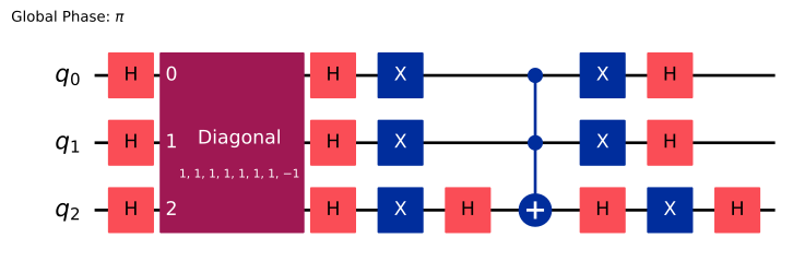
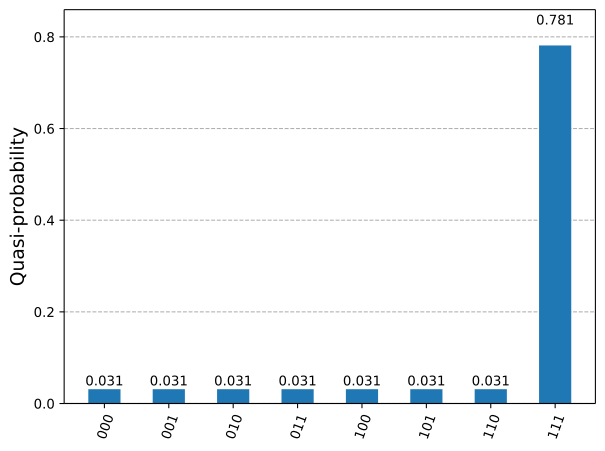
צרו Circuit קטן שה-Transpiler ינסה לייעל. דוגמה זו יוצרת Circuit המבצע את אלגוריתם גרובר עם אורקל שמסמן את המצב 111. לאחר מכן, סמלצו את ההתפלגות האידיאלית (מה שהייתם מצפים למדוד אם הייתם מריצים זאת על מחשב קוונטי מושלם אינסוף פעמים) לצורך השוואה בהמשך.

oracle = DiagonalGate([1] * 7 + [-1])
qc = QuantumCircuit(3)
qc.h([0, 1, 2])
qc = qc.compose(grover_operator(oracle))

qc.draw(output="mpl", style="iqp")

ideal_distribution = Statevector.from_instruction(qc).probabilities_dict()

plot_histogram(ideal_distribution)

טרנספילציה

כעת, בצעו טרנספילציה של ה-Circuits עבור ה-QPU. תשוו את ביצועי ה-Transpiler כשרמת optimization_level מוגדרת ל-0 (הנמוכה ביותר) לעומת 3 (הגבוהה ביותר). רמת האופטימיזציה הנמוכה ביותר עושה את המינימום ההכרחי כדי להפעיל את ה-Circuit על המכשיר; היא ממפה את ה-Qubits של ה-Circuit ל-Qubits של המכשיר ומוסיפה שערי SWAP כדי לאפשר את כל הפעולות דו-Qubit. רמת האופטימיזציה הגבוהה ביותר חכמה הרבה יותר ומשתמשת בהמון טריקים כדי להפחית את מספר ה-Gates הכולל. מכיוון שלשערים רב-Qubit יש שיעורי שגיאה גבוהים ו-Qubits מתנוונים עם הזמן, ה-Circuits הקצרים יותר אמורים לתת תוצאות טובות יותר.

important

דוגמה זו משתמשת בחומרת IBM Quantum®, אך ניתן לנסות אותה על כל QPU תואם-Qiskit. התוצאות שלכם עשויות להיות שונות.

התא הבא מבצע טרנספילציה של qc לשני ערכי optimization_level, מדפיס את מספר שערי ה-Qubit הכפול, ומוסיף את ה-Circuits המטרנספלים לרשימה. חלק מאלגוריתמי ה-Transpiler הם אקראיים, לכן מוגדר seed לצורך רבייה.

# Use Qiskit Runtime to run jobs on hardware
from qiskit_ibm_runtime import (
    QiskitRuntimeService,
    SamplerV2 as Sampler,
)

# Select the backend with the fewest number of jobs in the queue
service = QiskitRuntimeService()
backend = service.least_busy(
    operational=True, simulator=False, min_num_qubits=127
)
backend.name

'ibm_marrakesh'

# Need to add measurements to the circuit
qc.measure_all()

# Find the correct two-qubit gate
twoQ_gates = set(["ecr", "cz", "cx"])
for gate in backend.basis_gates:
    if gate in twoQ_gates:
        twoQ_gate = gate

circuits = []
for optimization_level in [0, 3]:
    pm = generate_preset_pass_manager(
        optimization_level, backend=backend, seed_transpiler=0
    )
    t_qc = pm.run(qc)
    print(
        f"Two-qubit gates (optimization_level={optimization_level}): ",
        t_qc.count_ops()[twoQ_gate],
    )
    circuits.append(t_qc)

Two-qubit gates (optimization_level=0):  21
Two-qubit gates (optimization_level=3):  12

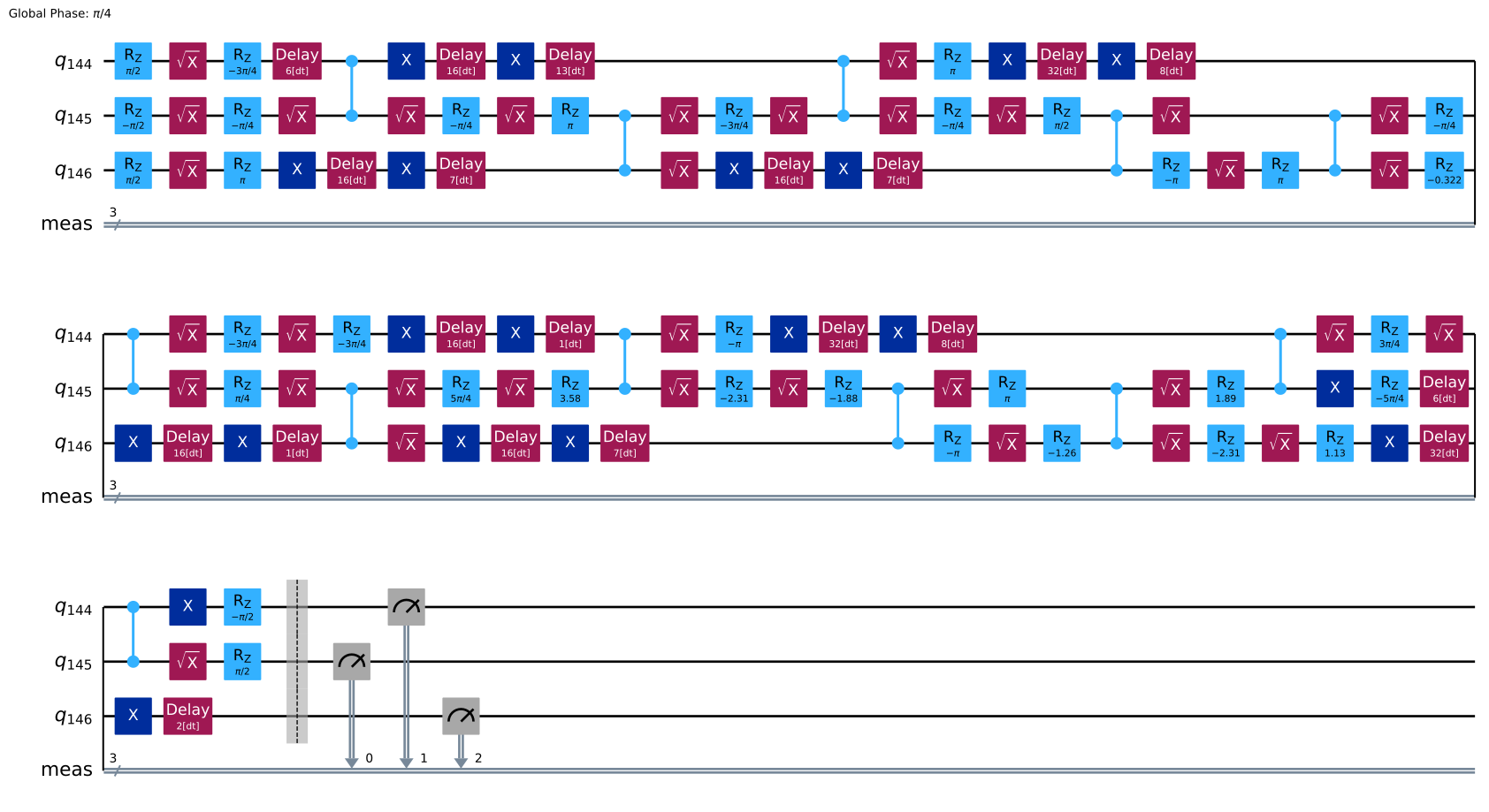
מכיוון ש-CNOTs בדרך כלל בעלי שיעור שגיאה גבוה, ה-Circuit שטורנספל עם optimization_level=3 אמור לפעול הרבה יותר טוב.

דרך נוספת לשפר ביצועים היא באמצעות dynamical decoupling, על-ידי הפעלת רצף של Gates על Qubits סרק. זה מבטל חלק מהאינטראקציות הלא-רצויות עם הסביבה. התא הבא מוסיף dynamic decoupling ל-Circuit שטורנספל עם optimization_level=3 ומוסיף אותו לרשימה.

from qiskit_ibm_runtime.transpiler.passes.scheduling import (
    ASAPScheduleAnalysis,
    PadDynamicalDecoupling,
)

# Get gate durations so the transpiler knows how long each operation takes
durations = backend.target.durations()

# This is the sequence we'll apply to idling qubits
dd_sequence = [XGate(), XGate()]

# Run scheduling and dynamic decoupling passes on circuit
pm = PassManager(
    [
        ASAPScheduleAnalysis(durations),
        PadDynamicalDecoupling(durations, dd_sequence),
    ]
)
circ_dd = pm.run(circuits[1])

# Add this new circuit to our list
circuits.append(circ_dd)

circ_dd.draw(output="mpl", style="iqp", idle_wires=False)

ביצוע ה-Circuit

בשלב זה, יש לכם רשימת Circuits מטרנספלים עם הגדרות שונות. כעת, הריצו את ה-Circuits האלה באמצעות ה-Sampler primitive ושמרו את התוצאות ב-result.

sampler = Sampler(backend)
job = sampler.run(
    [(circuit) for circuit in circuits],  # sample all three circuits
    shots=8000,
)
result = job.result()

צפייה בתוצאות

לבסוף, השוו את התוצאות מריצות המכשיר מול ההתפלגות האידיאלית. ניתן לראות שהתוצאות עם optimization_level=3 קרובות יותר להתפלגות האידיאלית בשל מספר ה-Gates הנמוך יותר, ו-optimization_level=3 + dd קרובה אף יותר בשל ה-dynamical decoupling.

binary_prob = [
    {
        k: v / res.data.meas.num_shots
        for k, v in res.data.meas.get_counts().items()
    }
    for res in result
]
plot_histogram(
    binary_prob + [ideal_distribution],
    bar_labels=False,
    legend=[
        "optimization_level=0",
        "optimization_level=3",
        "optimization_level=3 + dd",
        "ideal distribution",
    ],
)

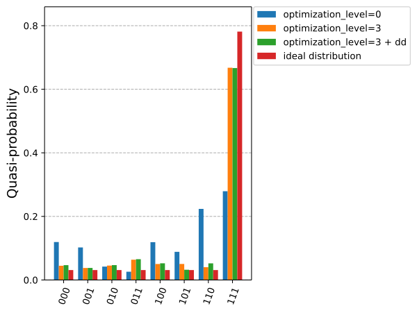
ניתן לאמת זאת על-ידי חישוב Hellinger fidelity בין כל קבוצת תוצאות לבין ההתפלגות האידיאלית (ערך גבוה יותר עדיף, ו-1 מייצג נאמנות מושלמת).

for prob in binary_prob:
    print(f"{hellinger_fidelity(prob, ideal_distribution):.3f}")

0.985
0.989
0.988

צעדים הבאים

המלצות

• חקרו כמה משאבי טרנספילציה מתקדמים, כגון:

  • כתיבת מעבר Transpiler מותאם אישית
  • יצירת טרנספילציה כנגד backends מותאמים אישית
  • התקנה ושימוש בתוספי Transpiler

• עיינו במדריכים הזמינים.