הפחתת שגיאות בקנה מידה של שירות עם הגברת שגיאות הסתברותית
אומדן שימוש: 14 דקות על מעבד Heron r3 (הערה: זהו אומדן בלבד. זמן הריצה בפועל עשוי להשתנות.)
תוצאות למידה
לאחר השלמת מדריך זה, המשתמשים אמורים להבין:
- את התיאוריה מאחורי אקסטרפולציה לאפס רעש (ZNE), השיטות השונות להגברת רעש, ומדוע הגברת שגיאות הסתברותית (PEA) עדיפה לניסויים בקנה מידה של שירות.
- כיצד לממש ZNE עם PEA בפועל באמצעות Qiskit.
דרישות מוקדמות
אנו ממליצים למשתמשים להכיר את הנושאים הבאים לפני עבודה עם מדריך זה:
- את שיעור הפחתת שגיאות של קורס Utility-scale quantum computing לידע בסיסי בשימוש בהפחתת שגיאות ב-Qiskit.
- את שיעור Utility-I של קורס Utility-scale quantum computing לרקע נוסף על הניסוי בקנה מידה של שירות המשמש כדוגמה במדריך זה.
רקע
מדריך זה מדגים כיצד להפעיל ניסוי הפחתת שגיאות בקנה מידה של שירות עם Qiskit Runtime, תוך שימוש בגרסה ניסויית של אקסטרפולציה לאפס רעש (ZNE) עם הגברת שגיאות הסתברותית (PEA).
 מקור: Y. Kim et al. Evidence for the utility of quantum computing before fault tolerance. Nature 618.7965 (2023)
אקסטרפולציה לאפס רעש (ZNE)
אקסטרפולציה לאפס רעש (ZNE) היא טכניקת הפחתת שגיאות המסירה את השפעות הרעש הבלתי ידוע במהלך הרצת Circuit, כאשר ניתן לשנות את עוצמת הרעש בדרך ידועה.
הטכניקה מניחה שערכי הציפייה משתנים עם הרעש לפי פונקציה ידועה:
כאשר מפרמטר את עוצמת הרעש וניתן להגביר אותה.
ניתן לממש ZNE בשלבים הבאים:
- הגברת רעש ה-Circuit עבור מספר גורמי רעש
- הרצת כל Circuit מוגבר-רעש למדידת
- אקסטרפולציה חזרה לגבול האפס-רעש

הגברת רעש עבור ZNE
האתגר המרכזי ביישום מוצלח של ZNE הוא לבנות מודל רעש מדויק עבור ערך הציפייה, ולהגביר את הרעש בדרך ידועה.
קיימות שלוש שיטות נפוצות להגברת שגיאות עבור ZNE:
| מתיחת פולס | קיפול Gate | הגברת שגיאות הסתברותית |
|---|---|---|
| הרחבת משך הפולס באמצעות כיול | חזרה על Gates במחזורי זהות | הוספת רעש על ידי דגימת ערוצי פאולי |
 |  |  |
| Kandala et al. Nature (2019) | Shultz et al. PRA (2022) | Li & Benjamin PRX (2017) |
| עבור ניסויים בקנה מידה של שירות, הגברת שגיאות הסתברותית (PEA) היא הגישה האטרקטיבית ביותר. |
- מתיחת פולס מניחה שרעש ה-Gate פרופורציונלי למשכו, דבר שאינו נכון בדרך כלל. בנוסף, הכיול יקר מבחינת משאבים.
- קיפול Gate דורש גורמי מתיחה גדולים המגבילים מאוד את עומק ה-Circuit שניתן להריץ.
- PEA ניתנת ליישום על כל Circuit שניתן להריץ עם גורם הרעש המקורי (), אך דורשת לימוד מודל הרעש.
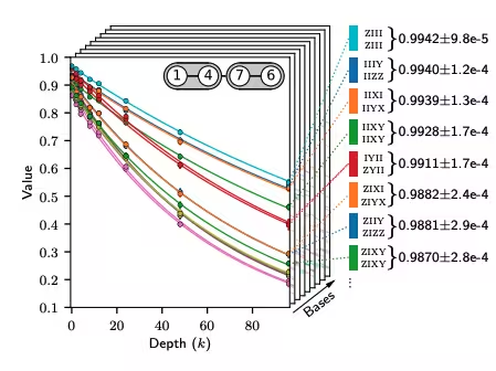
לימוד מודל הרעש עבור PEA
PEA מניחה את אותו מודל רעש מבוסס-שכבות כמו ביטול שגיאות הסתברותי (PEC); עם זאת, היא נמנעת מעומס הדגימה המתרחב אקספוננציאלית עם רעש ה-Circuit.
| שלב 1 | שלב 2 | שלב 3 |
|---|---|---|
| סיבוב פאולי של שכבות Gates דו-קיוביטיות | חזרה על זוגות זהות של שכבות ולמידת הרעש | גזירת ערך נאמנות (שגיאה לכל ערוץ רעש) |
 | 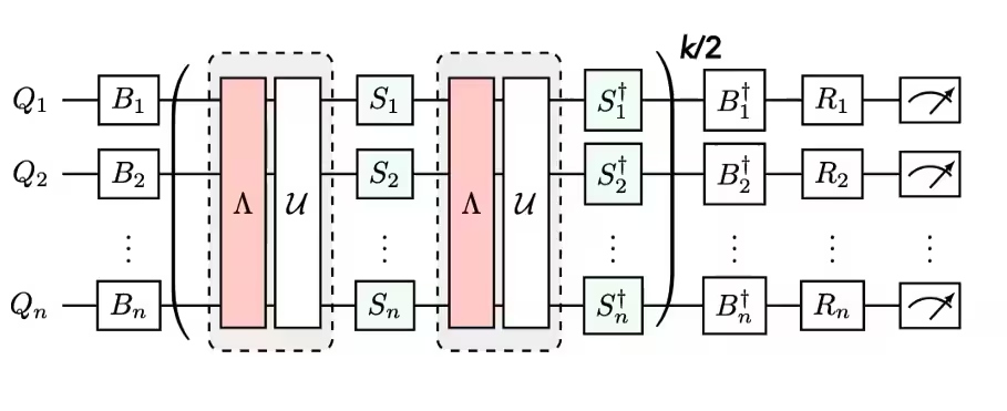 |  |
מקור: E. van den Berg, Z. Minev, A. Kandala, and K. Temme, Probabilistic error cancellation with sparse Pauli-Lindblad models on noisy quantum processors arXiv:2201.09866
דרישות מוקדמות
לפני תחילת מדריך זה, ודאו שהדברים הבאים מותקנים:
- Qiskit SDK גרסה 2.0 ומעלה, עם תמיכה בויזואליזציה
- Qiskit Runtime גרסה 0.22 ומעלה (
pip install qiskit-ibm-runtime)
הגדרה
בתא הבא, מייבאים חבילות רלוונטיות ויוצרים מספר פונקציות עזר לבניית ה-Circuits עבור התפתחות הזמן ב-Trotter של מודל איזינג הרוחבי דו-ממדי, בהתאמה לטופולוגיית ה-Backend.
# Added by doQumentation — required packages for this notebook
!pip install -q matplotlib numpy qiskit qiskit-ibm-runtime rustworkx
from __future__ import annotations
from collections.abc import Sequence
from collections import defaultdict
import numpy as np
import rustworkx
import matplotlib.pyplot as plt

from qiskit.circuit import QuantumCircuit, Parameter
from qiskit.circuit.library import CXGate, CZGate, ECRGate
from qiskit.providers import Backend
from qiskit.visualization import plot_error_map
from qiskit.transpiler.preset_passmanagers import generate_preset_pass_manager
from qiskit.quantum_info import SparsePauliOp
from qiskit.primitives import PubResult

from qiskit_ibm_runtime import QiskitRuntimeService
from qiskit_ibm_runtime import EstimatorV2 as Estimator

"""Trotter circuit generation"""

def remove_qubit_couplings(
    couplings: Sequence[tuple[int, int]], qubits: Sequence[int] | None = None
) -> list[tuple[int, int]]:
    """Remove qubits from a coupling list.

    Args:
        couplings: A sequence of qubit couplings.
        qubits: Optional, the qubits to remove.

    Returns:
        The input couplings with the specified qubits removed.
    """
    if qubits is None:
        return couplings
    qubits = set(qubits)
    return [edge for edge in couplings if not qubits.intersection(edge)]

def coupling_qubits(
    *couplings: Sequence[tuple[int, int]],
    allowed_qubits: Sequence[int] | None = None,
) -> list[int]:
    """Return a sorted list of all qubits involved in one or more couplings lists.

    Args:
        couplings: one or more coupling lists.
        allowed_qubits: Optional, the allowed qubits to include. If None all
            qubits are allowed.

    Returns:
        The intersection of all qubits in the couplings and the allowed qubits.
    """
    qubits = set()
    for edges in couplings:
        for edge in edges:
            qubits.update(edge)
    if allowed_qubits is not None:
        qubits = qubits.intersection(allowed_qubits)
    return list(qubits)

def construct_layer_couplings(
    backend: Backend,
) -> list[list[tuple[int, int]]]:
    """Separate a coupling map into disjoint 2-qubit gate layers.

    Args:
        backend: A backend to construct layer couplings for.

    Returns:
        A list of disjoint layers of directed couplings for the input coupling map.
    """
    coupling_graph = backend.coupling_map.graph.to_undirected(
        multigraph=False
    )
    edge_coloring = rustworkx.graph_bipartite_edge_color(coupling_graph)

    layers = defaultdict(list)
    for edge_idx, color in edge_coloring.items():
        layers[color].append(
            coupling_graph.get_edge_endpoints_by_index(edge_idx)
        )
    layers = [sorted(layers[i]) for i in sorted(layers.keys())]

    return layers

def entangling_layer(
    gate_2q: str,
    couplings: Sequence[tuple[int, int]],
    qubits: Sequence[int] | None = None,
) -> QuantumCircuit:
    """Generating a entangling layer for the specified couplings.

    This corresponds to a Trotter layer for a ZZ Ising term with angle Pi/2.

    Args:
        gate_2q: The 2-qubit basis gate for the layer, should be "cx", "cz", or "ecr".
        couplings: A sequence of qubit couplings to add CX gates to.
        qubits: Optional, the physical qubits for the layer. Any couplings involving
            qubits not in this list will be removed. If None the range up to the largest
            qubit in the couplings will be used.

    Returns:
        The QuantumCircuit for the entangling layer.
    """
    # Get qubits and convert to set to order
    if qubits is None:
        qubits = range(1 + max(coupling_qubits(couplings)))
    qubits = set(qubits)

    # Mapping of physical qubit to virtual qubit
    qubit_mapping = {q: i for i, q in enumerate(qubits)}

    # Convert couplings to indices for virtual qubits
    indices = [
        [qubit_mapping[i] for i in edge]
        for edge in couplings
        if qubits.issuperset(edge)
    ]

    # Layer circuit on virtual qubits
    circuit = QuantumCircuit(len(qubits))

    # Get 2-qubit basis gate and pre and post rotation circuits
    gate2q = None
    pre = QuantumCircuit(2)
    post = QuantumCircuit(2)

    if gate_2q == "cx":
        gate2q = CXGate()
        # Pre-rotation
        pre.sdg(0)
        pre.z(1)
        pre.sx(1)
        pre.s(1)
        # Post-rotation
        post.sdg(1)
        post.sxdg(1)
        post.s(1)
    elif gate_2q == "ecr":
        gate2q = ECRGate()
        # Pre-rotation
        pre.z(0)
        pre.s(1)
        pre.sx(1)
        pre.s(1)
        # Post-rotation
        post.x(0)
        post.sdg(1)
        post.sxdg(1)
        post.s(1)
    elif gate_2q == "cz":
        gate2q = CZGate()
        # Identity pre-rotation
        # Post-rotation
        post.sdg([0, 1])
    else:
        raise ValueError(
            f"Invalid 2-qubit basis gate {gate_2q}, should be 'cx', 'cz', or 'ecr'"
        )

    # Add 1Q pre-rotations
    for inds in indices:
        circuit.compose(pre, qubits=inds, inplace=True)

    # Use barriers around 2-qubit basis gate to specify a layer for PEA noise learning
    circuit.barrier()
    for inds in indices:
        circuit.append(gate2q, (inds[0], inds[1]))
    circuit.barrier()

    # Add 1Q post-rotations after barrier
    for inds in indices:
        circuit.compose(post, qubits=inds, inplace=True)

    # Add physical qubits as metadata
    circuit.metadata["physical_qubits"] = tuple(qubits)

    return circuit

def trotter_circuit(
    theta: Parameter | float,
    layer_couplings: Sequence[Sequence[tuple[int, int]]],
    num_steps: int,
    gate_2q: str | None = "cx",
    backend: Backend | None = None,
    qubits: Sequence[int] | None = None,
) -> QuantumCircuit:
    """Generate a Trotter circuit for the 2D Ising

    Args:
        theta: The angle parameter for X.
        layer_couplings: A list of couplings for each entangling layer.
        num_steps: the number of Trotter steps.
        gate_2q: The 2-qubit basis gate to use in entangling layers.
            Can be "cx", "cz", "ecr", or None if a backend is provided.
        backend: A backend to get the 2-qubit basis gate from, if provided
            will override the basis_gate field.
        qubits: Optional, the allowed physical qubits to truncate the
            couplings to. If None the range up to the largest
            qubit in the couplings will be used.

    Returns:
        The Trotter circuit.
    """
    if backend is not None:
        try:
            basis_gates = backend.configuration().basis_gates
        except AttributeError:
            basis_gates = backend.basis_gates
        for gate in ["cx", "cz", "ecr"]:
            if gate in basis_gates:
                gate_2q = gate
                break

    # If no qubits, get the largest qubit from all layers and
    # specify the range so the same one is used for all layers.
    if qubits is None:
        qubits = range(1 + max(coupling_qubits(layer_couplings)))

    # Generate the entangling layers
    layers = [
        entangling_layer(gate_2q, couplings, qubits=qubits)
        for couplings in layer_couplings
    ]

    # Construct the circuit for a single Trotter step
    num_qubits = len(qubits)
    trotter_step = QuantumCircuit(num_qubits)
    trotter_step.rx(theta, range(num_qubits))
    for layer in layers:
        trotter_step.compose(layer, range(num_qubits), inplace=True)

    # Construct the circuit for the specified number of Trotter steps
    circuit = QuantumCircuit(num_qubits)
    for _ in range(num_steps):
        circuit.rx(theta, range(num_qubits))
        for layer in layers:
            circuit.compose(layer, range(num_qubits), inplace=True)

    circuit.metadata["physical_qubits"] = tuple(qubits)
    return circuit

"""Result visualization functions"""

def plot_trotter_results(
    pub_result: PubResult,
    angles: Sequence[float],
    plot_noise_factors: Sequence[float] | None = None,
    plot_extrapolator: Sequence[str] | None = None,
    exact: np.ndarray = None,
    close: bool = True,
):
    """Plot average magnetization from ZNE result data.
    Args:
        pub_result: The Estimator PubResult for the PEA experiment.
        angles: The Rx angle values for the experiment.
        plot_raw: If provided plot the unextrapolated data for the noise factors.
        plot_extrapolator: If provided plot all extrapolators, if False only plot
            the Automatic method.
        exact: Optional, the exact values to include in the plot. Should be a 1D
            array-like where the values represent exact magnetization.
        close: Close the Matplotlib figure before returning.
    Returns:
        The figure.
    """
    data = pub_result.data

    evs = data.evs
    num_qubits = evs.shape[0]
    num_params = evs.shape[1]
    angles = np.asarray(angles).ravel()
    if angles.shape != (num_params,):
        raise ValueError(
            f"Incorrect number of angles for input data {angles.size} != {num_params}"
        )

    # Take average magnetization of qubits and its standard error
    x_vals = angles / np.pi
    y_vals = np.mean(evs, axis=0)
    y_errs = np.std(evs, axis=0) / np.sqrt(num_qubits)

    fig, _ = plt.subplots(1, 1)

    # Plot auto method
    plt.errorbar(x_vals, y_vals, y_errs, fmt="o-", label="ZNE (automatic)")

    # Plot individual extrapolator results
    if plot_extrapolator:
        y_vals_extrap = np.mean(data.evs_extrapolated, axis=0)
        y_errs_extrap = np.std(data.evs_extrapolated, axis=0) / np.sqrt(
            num_qubits
        )
        for i, extrap in enumerate(plot_extrapolator):
            plt.errorbar(
                x_vals,
                y_vals_extrap[:, i, 0],
                y_errs_extrap[:, i, 0],
                fmt="s-.",
                alpha=0.5,
                label=f"ZNE ({extrap})",
            )

    # Plot raw results
    if plot_noise_factors:
        y_vals_raw = np.mean(data.evs_noise_factors, axis=0)
        y_errs_raw = np.std(data.evs_noise_factors, axis=0) / np.sqrt(
            num_qubits
        )
        for i, nf in enumerate(plot_noise_factors):
            plt.errorbar(
                x_vals,
                y_vals_raw[:, i],
                y_errs_raw[:, i],
                fmt="d:",
                alpha=0.5,
                label=f"Raw (nf={nf:.1f})",
            )

    # Plot exact data
    if exact is not None:
        plt.plot(x_vals, exact, "--", color="black", alpha=0.5, label="Exact")

    plt.ylim(-0.1, 1.2)
    plt.xlabel("θ/π")
    plt.ylabel(r"$\overline{\langle Z \rangle}$")
    plt.legend()
    plt.title(
        f"Error Mitigated Average Magnetization for Rx(θ) [{num_qubits}-qubit]"
    )
    if close:
        plt.close(fig)
    return fig

def plot_qubit_zne_data(
    pub_result: PubResult,
    angles: Sequence[float],
    qubit: int,
    noise_factors: Sequence[float],
    extrapolator: Sequence[str] | None = None,
    extrapolated_noise_factors: Sequence[float] | None = None,
    num_cols: int | None = None,
    close: bool = True,
):
    """Plot ZNE extrapolation data for specific virtual qubit
    Args:
        pub_result: The Estimator PubResult for the PEA experiment.
        angles: The Rx theta angles used for the experiment.
        qubit: The virtual qubit index to plot.
        noise_factors: the raw noise factors.
        extrapolator: The extrapolator metadata for multiple extrapolators.
        extrapolated_noise_factors: The noise factors used for extrapolation.
        num_cols: The number of columns for the generated subplots.
        close: Close the Matplotlib figure before returning.
    Returns:
        The Matplotlib figure.
    """
    data = pub_result.data

    evs_auto = data.evs[qubit]
    stds_auto = data.stds[qubit]
    evs_extrap = data.evs_extrapolated[qubit]
    stds_extrap = data.stds_extrapolated[qubit]
    evs_raw = data.evs_noise_factors[qubit]
    stds_raw = data.stds_noise_factors[qubit]

    num_params = evs_auto.shape[0]
    angles = np.asarray(angles).ravel()
    if angles.shape != (num_params,):
        raise ValueError(
            f"Incorrect number of angles for input data {angles.size} != {num_params}"
        )

    # Make a square subplot
    num_cols = num_cols or int(np.ceil(np.sqrt(num_params)))
    num_rows = int(np.ceil(num_params / num_cols))
    fig, axes = plt.subplots(
        num_rows, num_cols, sharex=True, sharey=True, figsize=(12, 5)
    )
    fig.suptitle(f"ZNE data for virtual qubit {qubit}")

    for pidx, ax in zip(range(num_params), axes.flat):
        # Plot auto extrapolated
        ax.errorbar(
            0,
            evs_auto[pidx],
            stds_auto[pidx],
            fmt="o",
            label="PEA (automatic)",
        )

        # Plot extrapolators
        if (
            extrapolator is not None
            and extrapolated_noise_factors is not None
        ):
            for i, method in enumerate(extrapolator):
                ax.errorbar(
                    extrapolated_noise_factors,
                    evs_extrap[pidx, i],
                    stds_extrap[pidx, i],
                    fmt="-",
                    alpha=0.5,
                    label=f"PEA ({method})",
                )

        # Plot raw
        ax.errorbar(
            noise_factors, evs_raw[pidx], stds_raw[pidx], fmt="d", label="Raw"
        )

        ax.set_yticks([0, 0.5, 1, 1.5, 2])
        ax.set_ylim(0, max(1, 1.1 * max(evs_auto)))

        ax.set_xticks([0, *noise_factors])
        ax.set_title(f"θ/π = {angles[pidx]/np.pi:.2f}")
        if pidx == 0:
            ax.set_ylabel(r"$\langle Z_{" + str(qubit) + r"} \rangle$")
        if pidx == num_params - 1:
            ax.set_xlabel("Noise Factor")
            ax.legend()
    plt.tight_layout()
    if close:
        plt.close(fig)
    return fig
דוגמה בסימולטור בקנה מידה קטן
נדלג על שלב זה מכיוון שהפחתת שגיאות בזמן ריצה אינה נתמכת בסימולטורים.
דוגמה בחומרה אמיתית בקנה מידה גדול
שלב 1: מיפוי קלטים קלאסיים לבעיה קוונטית
יצירת Circuit מפורמטר של מודל איזינג
בחירת Backend
ראשית, בחרו Backend להרצה. הדגמה זו מתבצעת על Backend בעל 127 קיוביטים, אך ניתן לשנות זאת לכל Backend הזמין לכם.
service = QiskitRuntimeService()
backend = service.least_busy(
    operational=True, simulator=False, min_num_qubits=127
)
backend
<IBMBackend('ibm_fez')>
הגדרת קישורי שכבת השזירה
כדי לממש את סימולציית איזינג ב-Trotter, הגדירו שלוש שכבות של קישורי Gate דו-קיוביטי עבור המכשיר, אשר יחזרו על עצמן בכל אחד משלבי Trotter. שכבות אלו מגדירות את שלוש השכבות המסובבות שנדרש ללמוד עבורן את הרעש לצורך יישום ההפחתה.
layer_couplings = construct_layer_couplings(backend)
for i, layer in enumerate(layer_couplings):
    print(f"Layer {i}:\n{layer}\n")
Layer 0:
[(2, 3), (4, 5), (6, 7), (8, 9), (10, 11), (12, 13), (14, 15), (16, 23), (18, 31), (19, 35), (20, 21), (25, 37), (26, 27), (28, 29), (33, 39), (36, 41), (38, 49), (42, 43), (45, 46), (47, 57), (51, 52), (53, 54), (56, 63), (58, 71), (59, 75), (61, 62), (64, 65), (66, 67), (68, 69), (72, 73), (76, 81), (79, 93), (82, 83), (84, 85), (86, 87), (88, 89), (91, 98), (94, 95), (97, 107), (99, 115), (100, 101), (102, 103), (105, 117), (108, 109), (110, 111), (113, 114), (116, 121), (118, 129), (123, 136), (124, 125), (126, 127), (130, 131), (132, 133), (135, 139), (138, 151), (142, 143), (144, 145), (146, 147), (152, 153), (154, 155)]

Layer 1:
[(0, 1), (3, 16), (5, 6), (7, 8), (11, 18), (13, 14), (17, 27), (21, 22), (23, 24), (25, 26), (29, 38), (30, 31), (32, 33), (34, 35), (39, 53), (41, 42), (43, 56), (44, 45), (47, 48), (49, 50), (51, 58), (54, 55), (57, 67), (60, 61), (62, 63), (65, 66), (69, 78), (70, 71), (73, 79), (74, 75), (77, 85), (80, 81), (83, 84), (87, 97), (89, 90), (91, 92), (93, 94), (96, 103), (101, 116), (104, 105), (106, 107), (109, 118), (111, 112), (113, 119), (114, 115), (117, 125), (121, 122), (123, 124), (127, 137), (128, 129), (131, 138), (133, 134), (136, 143), (139, 155), (140, 141), (145, 146), (147, 148), (149, 150), (151, 152)]

Layer 2:
[(1, 2), (3, 4), (7, 17), (9, 10), (11, 12), (15, 19), (21, 36), (22, 23), (24, 25), (27, 28), (29, 30), (31, 32), (33, 34), (37, 45), (40, 41), (43, 44), (46, 47), (48, 49), (50, 51), (52, 53), (55, 59), (61, 76), (63, 64), (65, 77), (67, 68), (69, 70), (71, 72), (73, 74), (78, 89), (81, 82), (83, 96), (85, 86), (87, 88), (90, 91), (92, 93), (95, 99), (98, 111), (101, 102), (103, 104), (105, 106), (107, 108), (109, 110), (112, 113), (119, 133), (120, 121), (122, 123), (125, 126), (127, 128), (129, 130), (131, 132), (134, 135), (137, 147), (141, 142), (143, 144), (148, 149), (150, 151), (153, 154)]
הסרת קיוביטים פגומים
בחנו את מפת הקישוריות של ה-Backend וזהו קיוביטים המחוברים לקישורים בעלי שגיאה גבוהה. הסירו קיוביטים "פגומים" אלו מהניסוי.
# Plot gate error map
# NOTE: These can change over time, so your results may look different
plot_error_map(backend)
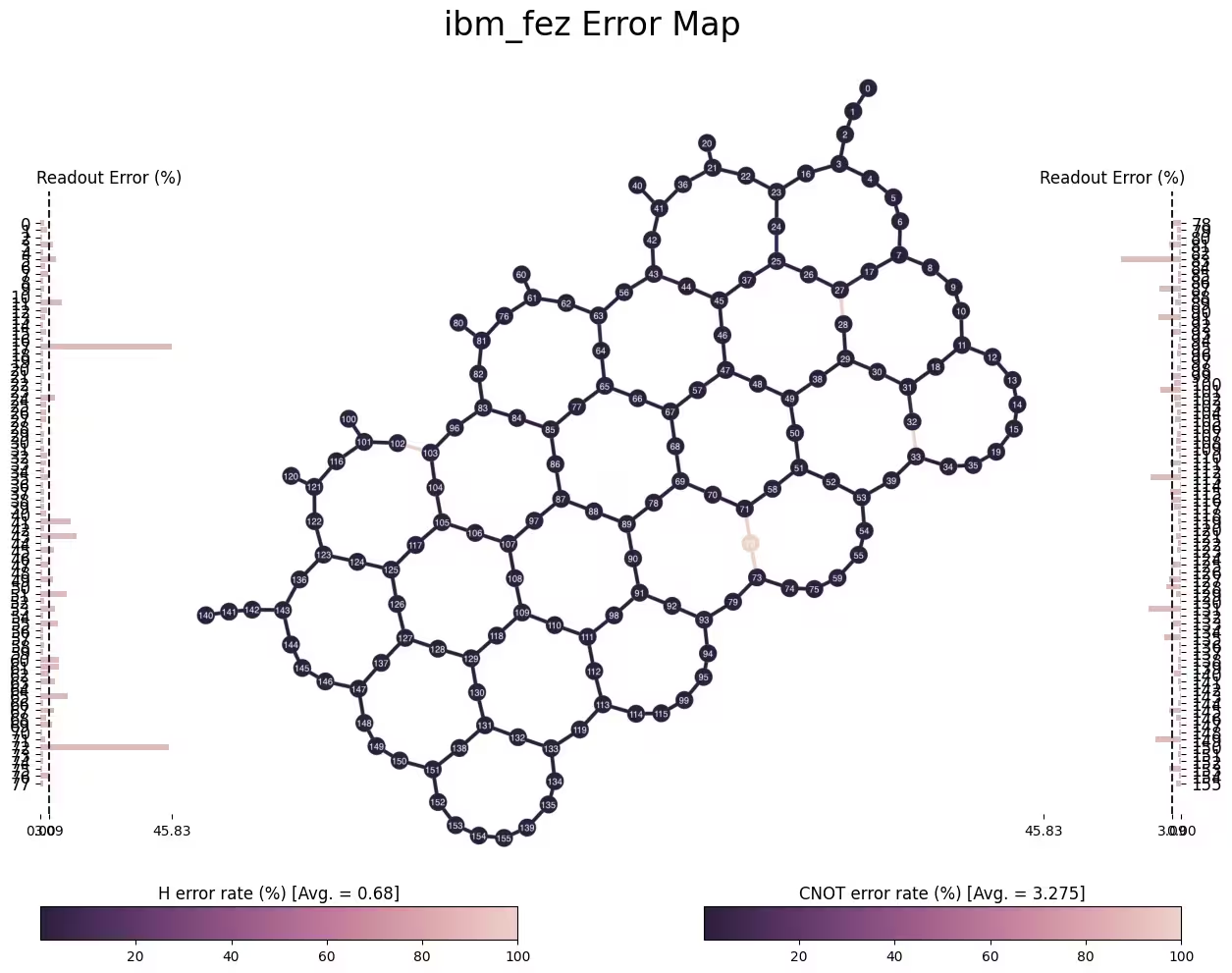
bad_qubits = {
    32,
    33,
    71,
    72,
    73,
    102,
    103,
}  # qubits removed based on high coupling error (1.00)
good_qubits = list(set(range(backend.num_qubits)).difference(bad_qubits))
print("Physical qubits:\n", good_qubits)
Physical qubits:
 [0, 1, 2, 3, 4, 5, 6, 7, 8, 9, 10, 11, 12, 13, 14, 15, 16, 17, 18, 19, 20, 21, 22, 23, 24, 25, 26, 27, 28, 29, 30, 31, 34, 35, 36, 37, 38, 39, 40, 41, 42, 43, 44, 45, 46, 47, 48, 49, 50, 51, 52, 53, 54, 55, 56, 57, 58, 59, 60, 61, 62, 63, 64, 65, 66, 67, 68, 69, 70, 74, 75, 76, 77, 78, 79, 80, 81, 82, 83, 84, 85, 86, 87, 88, 89, 90, 91, 92, 93, 94, 95, 96, 97, 98, 99, 100, 101, 104, 105, 106, 107, 108, 109, 110, 111, 112, 113, 114, 115, 116, 117, 118, 119, 120, 121, 122, 123, 124, 125, 126, 127, 128, 129, 130, 131, 132, 133, 134, 135, 136, 137, 138, 139, 140, 141, 142, 143, 144, 145, 146, 147, 148, 149, 150, 151, 152, 153, 154, 155]
יצירת Circuit ה-Trotter הראשי
num_steps = 6
theta = Parameter("theta")
circuit = trotter_circuit(
    theta, layer_couplings, num_steps, qubits=good_qubits, backend=backend
)
יצירת רשימת ערכי פרמטרים להקצאה מאוחרת
num_params = 12

# 12 parameter values for Rx between [0, pi/2].
# Reshape to outer product broadcast with observables
parameter_values = np.linspace(0, np.pi / 2, num_params).reshape(
    (num_params, 1)
)
num_params = parameter_values.size
שלב 2: אופטימיזציה של הבעיה לביצוע על חומרת קוונטום
מעגל ISA
לפני הרצת המעגל על חומרה, יש לבצע אופטימיזציה לביצוע על החומרה. תהליך זה כולל מספר שלבים:
- בחירת פריסת קיוביטים (qubit layout) שממפה את הקיוביטים הווירטואליים של המעגל לקיוביטים פיזיים על החומרה.
- הוספת שערי החלפה (swap gates) לפי הצורך, כדי לנתב אינטראקציות בין קיוביטים שאינם מחוברים.
- תרגום השערים במעגל להוראות ארכיטקטורת מערכת הוראות (ISA) שניתן להריץ ישירות על החומרה.
- ביצוע אופטימיזציות מעגל כדי למזער את עומק המעגל ואת מספר השערים.
אמנם ה-Transpiler המובנה ב-Qiskit מסוגל לבצע את כל השלבים הללו, אולם מדריך זה מדגים בניית מעגל Trotter בסדר גודל שימוש-מלא מהיסוד. יש לבחור את הקיוביטים הפיזיים הטובים ולהגדיר שכבות שזירה על זוגות קיוביטים מחוברים מתוך הקיוביטים שנבחרו. עם זאת, עדיין יש צורך לתרגם שערים שאינם ISA במעגל ולנצל את כל אופטימיזציות המעגל שמציע ה-Transpiler.
יש לבצע transpile למעגל עבור ה-Backend שנבחר, על ידי יצירת pass manager והרצתו על המעגל. כמו כן, יש לקבע את הפריסה הראשונית של המעגל ל-good_qubits שכבר נבחרו. דרך נוחה ליצור pass manager היא להשתמש בפונקציה generate_preset_pass_manager. ראו ב-Transpile with pass managers להסבר מפורט יותר על Transpiling עם pass managers.
pm = generate_preset_pass_manager(
    backend=backend,
    initial_layout=good_qubits,
    layout_method="trivial",
    optimization_level=1,
)

isa_circuit = pm.run(circuit)
Observable-ים מסוג ISA
כעת, יש ליצור את כל ה-Observable-ים מסוג ממשקל 1 עבור כל קיוביט וירטואלי, על ידי ריפוד של המספר הדרוש של איברי .
observables = []
num_qubits = len(good_qubits)
for q in range(num_qubits):
    observables.append(
        SparsePauliOp("I" * (num_qubits - q - 1) + "Z" + "I" * q)
    )
תהליך ה-Transpilation מיפה את הקיוביטים הווירטואליים של המעגל לקיוביטים פיזיים על החומרה. המידע על פריסת הקיוביטים מאוחסן במאפיין layout של המעגל שעבר transpilation. ה-Observable גם הוא מוגדר במונחים של הקיוביטים הווירטואליים, לכן יש להחיל פריסה זו על ה-Observable. זה נעשה באמצעות מתודת apply_layout של SparsePauliOp.
שימו לב שכל observable עטוף ברשימה בבלוק הקוד הבא. הדבר נעשה כדי לבצע broadcast עם ערכי הפרמטרים, כך שכל observable של קיוביט ייוכד עבור כל ערך theta. כללי ה-broadcasting עבור primitives ניתן למצוא כאן.
isa_observables = [
    [obs.apply_layout(layout=isa_circuit.layout)] for obs in observables
]
שלב 3: ביצוע באמצעות Primitives של Qiskit
pub = (isa_circuit, isa_observables, parameter_values)
הגדרת אפשרויות Estimator
כעת יש להגדיר את אפשרויות ה-Estimator הדרושות להרצת ניסוי הפחתת השגיאות. זה כולל אפשרויות ללמידת הרעש של שכבות השזירה ולאקסטרפולציה מסוג ZNE.
אנחנו משתמשים בתצורה הבאה:
# Experiment options
num_randomizations = 700
num_randomizations_learning = 40
max_batch_circuits = 3 * num_params
shots_per_randomization = 64
learning_pair_depths = [0, 1, 2, 4, 6, 12, 24]
noise_factors = [1, 1.3, 1.6]
extrapolated_noise_factors = np.linspace(0, max(noise_factors), 20)

# Base option formatting
options = {
    # Builtin resilience settings for ZNE
    "resilience": {
        "measure_mitigation": True,
        "zne_mitigation": True,
        # TREX noise learning configuration
        "measure_noise_learning": {
            "num_randomizations": num_randomizations_learning,
            "shots_per_randomization": 1024,
        },
        # PEA noise model configuration
        "layer_noise_learning": {
            "max_layers_to_learn": 3,
            "layer_pair_depths": learning_pair_depths,
            "shots_per_randomization": shots_per_randomization,
            "num_randomizations": num_randomizations_learning,
        },
        "zne": {
            "amplifier": "pea",
            "noise_factors": noise_factors,
            "extrapolator": ("exponential", "linear"),
            "extrapolated_noise_factors": extrapolated_noise_factors.tolist(),
        },
    },
    # Randomization configuration
    "twirling": {
        "num_randomizations": num_randomizations,
        "shots_per_randomization": shots_per_randomization,
        "strategy": "active-circuit",
    },
    # Optional Dynamical Decoupling (DD)
    "dynamical_decoupling": {"enable": True, "sequence_type": "XY4"},
    # Job tag
    "environment": {"job_tags": ["TUT_PEA"]},
}
הסבר על אפשרויות ZNE
להלן פרטים על האפשרויות הנוספות בגרסה הניסיונית. שימו לב שאפשרויות ושמות אלו אינם סופיים, וכל מה שכאן עשוי להשתנות לפני שחרור רשמי.
- amplifier: השיטה שתשמש להגברת הרעש עד לגורמי הרעש המיועדים.
הערכים המותרים הם
"gate_folding", שמגביר על ידי חזרה על שערי בסיס דו-קיוביט, ו-"pea", שמגביר על ידי דגימה הסתברותית לאחר למידת מודל הרעש מסוג Pauli-twirled עבור שכבות של שערי בסיס דו-קיוביט בעלי Pauli-twirling. קיימות גם אפשרויות"gate_folding_front"ו-"gate_folding_back"המוסברות בתיעוד ה-API - extrapolated_noise_factors: יש לציין ערך אחד או יותר של גורם רעש שבהם יש להעריך את המודלים המוחצנים. אם מדובר ברצף ערכים, התוצאות שיוחזרו יהיו מערכיות עם גורם הרעש המצוין המוערך עבור מודל האקסטרפולציה. ערך של 0 מתאים לאקסטרפולציה לאפס-רעש.
הרצת הניסוי
estimator = Estimator(mode=backend, options=options)
job = estimator.run([pub])
print(f"Job ID {job.job_id()}")
Job ID d7fa8oe2cugc739qbb10
job.status()
'DONE'
שלב 4: עיבוד-לאחר והחזרת התוצאה בפורמט קלאסי הרצוי
לאחר סיום הניסוי, ניתן לצפות בתוצאות. מאחזרים את ערכי הציפייה הגולמיים והמופחתים ומשווים אותם לתוצאות המדויקות. לאחר מכן, מציגים גרפית את ערכי הציפייה — הן המופחתים (מוחצנים) והן הגולמיים — כממוצע על פני כל הקיוביטים עבור כל פרמטר. לבסוף, מציגים גרפית ערכי ציפייה עבור קיוביטים בודדים לפי בחירתכם.
primitive_result = job.result()
צורות תוצאה כלליות ומטא-נתונים
האובייקט PrimitiveResult מכיל מבנה דמוי-רשימה בשם PubResult. מאחר שאנו שולחים רק PUB אחד ל-Estimator, ה-PrimitiveResult מכיל אובייקט PubResult בודד.
ערכי הציפייה ושגיאות התקן של תוצאת ה-PUB (primitive unified bloc) הם בעלי ערכים מערכיים. עבור עבודות Estimator עם ZNE, קיימים מספר שדות נתונים של ערכי ציפייה ושגיאות תקן הזמינים במיכל DataBin של PubResult. נדון בקצרה בשדות הנתונים של ערכי הציפייה כאן (שדות נתונים דומים זמינים גם עבור שגיאות תקן (stds)).
pub_result.data.evs: ערכי ציפייה המתאימים לאפס-רעש (מבוססים על האקסטרפולציה הטובה ביותר הוריסטית).- הציר הראשון הוא אינדקס הקיוביט הווירטואלי עבור ה-observable ( קיוביטים וירטואליים/observable-ים)
- הציר השני מאנדקס את ערך הפרמטר עבור ( ערכי פרמטר)
pub_result.data.evs_extrapolated: ערכי ציפייה עבור גורמי רעש מוחצנים לכל מחצין. למערך זה שני צירים נוספים.- הציר השלישי מאנדקס את שיטות האקסטרפולציה ( מחצינים,
exponentialו-linear) - הציר האחרון מאנדקס את
extrapolated_noise_factors( נקודות אקסטרפולציה שצוינו באפשרות)
- הציר השלישי מאנדקס את שיטות האקסטרפולציה ( מחצינים,
pub_result.data.evs_noise_factors: ערכי ציפייה גולמיים עבור כל גורם רעש.- הציר השלישי מאנדקס את
noise_factorsהגולמיים ( גורמים)
- הציר השלישי מאנדקס את
pub_result = primitive_result[0]

print(
    f"{pub_result.data.evs.shape=}\n"
    f"{pub_result.data.evs_extrapolated.shape=}\n"
    f"{pub_result.data.evs_noise_factors.shape=}\n"
)
pub_result.data.evs.shape=(149, 12)
pub_result.data.evs_extrapolated.shape=(149, 12, 2, 20)
pub_result.data.evs_noise_factors.shape=(149, 12, 3)
מספר שדות מטא-נתונים זמינים גם ב-PrimitiveResult. המטא-נתונים כוללים:
resilience/zne/noise_factors: גורמי הרעש הגולמייםresilience/zne/extrapolator: המחצינים (extrapolators) שנעשה בהם שימוש עבור כל תוצאה
primitive_result.metadata
{'dynamical_decoupling': {'enable': True,
  'sequence_type': 'XY4',
  'extra_slack_distribution': 'middle',
  'scheduling_method': 'alap'},
 'twirling': {'enable_gates': True,
  'enable_measure': True,
  'num_randomizations': 700,
  'shots_per_randomization': 64,
  'interleave_randomizations': True,
  'strategy': 'active-circuit'},
 'resilience': {'measure_mitigation': True,
  'zne_mitigation': True,
  'pec_mitigation': False,
  'zne': {'noise_factors': [1.0, 1.3, 1.6],
   'extrapolator': ['exponential', 'linear'],
   'extrapolated_noise_factors': [0.0,
    0.08421052631578947,
    0.16842105263157894,
    0.25263157894736843,
    0.3368421052631579,
    0.42105263157894735,
    0.5052631578947369,
    0.5894736842105263,
    0.6736842105263158,
    0.7578947368421053,
    0.8421052631578947,
    0.9263157894736842,
    1.0105263157894737,
    1.0947368421052632,
    1.1789473684210525,
    1.263157894736842,
    1.3473684210526315,
    1.431578947368421,
    1.5157894736842106,
    1.6]},
  'layer_noise_model': [LayerError(circuit=<qiskit.circuit.quantumcircuit.QuantumCircuit object at 0x1354890f0>, qubits=[0, 1, 2, 3, 4, 5, 6, 7, 8, 9, 10, 11, 12, 13, 14, 15, 16, 17, 18, 19, 20, 21, 22, 23, 24, 25, 26, 27, 28, 29, 30, 31, 34, 35, 36, 37, 38, 39, 40, 41, 42, 43, 44, 45, 46, 47, 48, 49, 50, 51, 52, 53, 54, 55, 56, 57, 58, 59, 60, 61, 62, 63, 64, 65, 66, 67, 68, 69, 70, 74, 75, 76, 77, 78, 79, 80, 81, 82, 83, 84, 85, 86, 87, 88, 89, 90, 91, 92, 93, 94, 95, 96, 97, 98, 99, 100, 101, 104, 105, 106, 107, 108, 109, 110, 111, 112, 113, 114, 115, 116, 117, 118, 119, 120, 121, 122, 123, 124, 125, 126, 127, 128, 129, 130, 131, 132, 133, 134, 135, 136, 137, 138, 139, 140, 141, 142, 143, 144, 145, 146, 147, 148, 149, 150, 151, 152, 153, 154, 155], error=PauliLindbladError(generators=['IIIIIIIIIIIIIIIIIIIIIIIIIIIIIIIIIIIIIIIIIIIIIIIIII...',
    'IIIIIIIIIIIIIIIIIIIIIIIIIIIIIIIIIIIIIIIIIIIIIIIIII...',
    'IIIIIIIIIIIIIIIIIIIIIIIIIIIIIIIIIIIIIIIIIIIIIIIIII...',
    'IIIIIIIIIIIIIIIIIIIIIIIIIIIIIIIIIIIIIIIIIIIIIIIIII...',
    'IIIIIIIIIIIIIIIIIIIIIIIIIIIIIIIIIIIIIIIIIIIIIIIIII...',
    'IIIIIIIIIIIIIIIIIIIIIIIIIIIIIIIIIIIIIIIIIIIIIIIIII...',
    'IIIIIIIIIIIIIIIIIIIIIIIIIIIIIIIIIIIIIIIIIIIIIIIIII...',
    'IIIIIIIIIIIIIIIIIIIIIIIIIIIIIIIIIIIIIIIIIIIIIIIIII...',
    'IIIIIIIIIIIIIIIIIIIIIIIIIIIIIIIIIIIIIIIIIIIIIIIIII...',
    'IIIIIIIIIIIIIIIIIIIIIIIIIIIIIIIIIIIIIIIIIIIIIIIIII...',
    'IIIIIIIIIIIIIIIIIIIIIIIIIIIIIIIIIIIIIIIIIIIIIIIIII...',
    'IIIIIIIIIIIIIIIIIIIIIIIIIIIIIIIIIIIIIIIIIIIIIIIIII...',
    'IIIIIIIIIIIIIIIIIIIIIIIIIIIIIIIIIIIIIIIIIIIIIIIIII...', ...], rates=[0.00155, 0.00144, 0.00637, 0.00023, 0.0, 0.0, 0.00018, 0.00035, 0.0, 0.00014, 5e-05, 0.00041, 0.0, 0.0, 0.0, 0.0001, 0.0001, 0.0, 9e-05, 6e-05, 0.0, 7e-05, 0.0001, 0.00013, 0.00018, 1e-05, 5e-05, 7e-05, 6e-05, 6e-05, 0.00029, 0.00016, 6e-05, 6e-05, 0.00046, 0.00073, 0.00031, 0.00025, 0.00018, 0.00022, 0.0, 8e-05, 0.00012, 0.00015, 0.00012, 0.0, 0.0, 0.00023, 5e-05, 5e-05, 7e-05, 0.00064, 4e-05, 2e-05, 0.00072, 0.00037, 2e-05, 4e-05, 0.00077, 0.0003, 0.00042, 0.00027, 0.00016, 0.0, 8e-05, 5e-05, 0.00019, 0.0, 0.0, 0.00021, 0.00014, 0.00061, 0.0, 0.00016, 3e-05, 0.00053, 0.00013, 0.0, 0.00068, 0.00011, 0.0, 0.00013, 0.00078, 0.01885, 0.00032, 0.00034, 0.00035, 0.00052, 3e-05, 0.0, 0.0, 0.0, 0.0, 0.0, 0.00028, 0.00123, 0.0, 0.0, 0.0, 0.00034, 0.00011, 0.0001, 0.00076, 0.00041, 0.0001, 0.00011, 0.00082, 0.0, 0.00066, 0.0, 0.00055, 7e-05, 0.00018, 0.00011, 0.00024, 3e-05, 0.00015, 0.00014, 0.0, 0.00076, 9e-05, 0.00016, 8e-05, 0.00132, 0.0, 0.00019, 0.00215, 0.00109, 0.00019, 0.0, 0.00201, 0.00021, 0.0006, 0.00032, 0.00046, 0.00027, 0.0, 8e-05, 0.0001, 0.00027, 0.0, 0.00015, 0.00018, 0.0, 0.00026, 0.00024, 5e-05, 0.00031, 0.0, 0.00034, 0.00039, 9e-05, 0.00034, 0.0, 0.00078, 0.00794, 0.00045, 0.00061, 0.00066, 0.0, 0.0, 0.00032, 6e-05, 5e-05, 7e-05, 0.0, 0.0001, 0.00036, 0.0, 0.00037, 0.00013, 0.00016, 3e-05, 8e-05, 0.00067, 0.00024, 8e-05, 3e-05, 0.00074, 0.00224, 0.00029, 0.00026, 0.00031, 0.00076, 5e-05, 0.0, 2e-05, 0.00072, 0.0, 1e-05, 0.00011, 0.00027, 0.0, 0.00017, 0.0, 0.0, 0.00012, 0.0, 0.0, 0.0, 0.0, 0.00067, 0.00063, 0.0, 0.0, 0.0, 0.00102, 0.0, 0.00011, 0.00026, 4e-05, 1e-05, 0.0002, 0.0, 0.00011, 0.0, 0.00021, 0.00015, 0.0005, 0.00011, 0.00013, 0.0, 0.0002, 0.00016, 0.00015, 8e-05, 2e-05, 7e-05, 0.00023, 0.00042, 0.0, 0.00049, 0.00056, 0.00372, 0.00017, 0.00012, 0.0, 0.00026, 0.00021, 0.0, 0.00012, 0.00046, 0.00305, 0.0005, 0.00057, 9e-05, 0.0009, 0.0, 7e-05, 0.00011, 0.00084, 0.0, 0.0, 0.0001, 0.00067, 0.0, 0.0, 0.0, 4e-05, 0.0, 1e-05, 0.00053, 0.0, 9e-05, 0.00021, 0.0, 1e-05, 0.0, 8e-05, 0.0, 0.0, 0.0, 9e-05, 0.00083, 0.00084, 0.00038, 9e-05, 3e-05, 0.00039, 0.02059, 0.0, 0.0, 0.0, 0.01787, 0.00012, 0.00024, 0.0, 0.00401, 0.0, 0.0, 0.0, 4e-05, 0.0, 0.0, 0.00018, 0.0, 0.00031, 0.00018, 0.0, 0.0, 0.0, 0.0, 0.00013, 0.0, 0.00027, 1e-05, 0.0, 0.00021, 0.0, 0.0, 0.00029, 0.00159, 0.0, 0.0, 0.00052, 0.0079, 0.0, 0.0002, 0.00147, 0.00048, 4e-05, 0.00976, 0.00957, 0.0011, 0.0, 0.0, 4e-05, 0.00048, 0.01068, 0.00487, 0.00225, 0.0, 0.0, 0.00026, 0.00052, 0.00033, 0.0, 0.00019, 0.0, 0.0, 0.00038, 0.0, 0.0, 0.0, 0.00154, 0.0, 0.0, 0.0, 0.00046, 0.0, 9e-05, 0.00077, 0.0002, 9e-05, 0.0, 0.00077, 0.00061, 6e-05, 0.00045, 0.00081, 0.00016, 0.0, 0.0, 0.0001, 0.00064, 4e-05, 0.0002, 0.0, 0.00056, 7e-05, 0.0, 0.0, 0.00066, 5e-05, 0.00025, 0.00077, 0.00011, 0.0, 0.0, 0.00065, 0.00025, 5e-05, 0.00082, 6e-05, 0.0, 0.00011, 0.00354, 0.00027, 0.00039, 0.00046, 0.00014, 0.0, 0.00013, 0.00067, 0.00064, 0.0006, 0.00053, 2e-05, 0.00016, 0.00067, 0.0, 0.00013, 0.0, 0.00047, 0.00016, 2e-05, 0.00067, 4e-05, 0.0, 0.00015, 0.00028, 0.00044, 0.00041, 0.00014, 0.00011, 0.0, 0.0, 5e-05, 0.0, 0.00017, 0.00022, 9e-05, 6e-05, 0.0, 0.00021, 0.0007, 3e-05, 0.0, 0.0, 0.0002, 0.00012, 3e-05, 0.0002, 0.0001, 3e-05, 0.00012, 0.00026, 0.00033, 0.00053, 0.00037, 0.00039, 9e-05, 6e-05, 7e-05, 0.00012, 0.00012, 0.0, 0.00022, 0.0, 0.00034, 0.00014, 8e-05, 0.0001, 0.00179, 0.00186, 0.00096, 0.00028, 0.00051, 0.00033, 0.0, 0.0, 0.00015, 0.0004, 0.0, 8e-05, 0.00015, 2e-05, 0.00015, 0.0, 0.00045, 0.0002, 0.0, 0.0, 0.00063, 0.00044, 0.00036, 0.00064, 0.0003, 2e-05, 0.0, 0.00124, 0.0, 0.0, 0.0, 0.00169, 0.00032, 0.00018, 0.0, 0.00147, 0.0, 0.0, 0.00037, 0.00095, 0.0, 0.00051, 0.00182, 0.00088, 0.00051, 0.0, 0.00116, 0.00093, 0.00124, 0.00219, 0.00052, 0.00072, 4e-05, 0.0, 0.0, 4e-05, 0.0, 0.00025, 0.00013, 0.0001, 0.00031, 0.0, 0.00027, 0.00022, 0.0, 0.00016, 0.0, 1e-05, 0.0001, 0.0, 3e-05, 0.0, 0.0, 2e-05, 6e-05, 0.0, 0.00021, 0.00251, 0.0, 0.0, 7e-05, 0.0, 0.0, 0.0, 0.00047, 5e-05, 2e-05, 0.00062, 0.00038, 2e-05, 5e-05, 0.00055, 0.00125, 0.00049, 0.00033, 0.00031, 0.00015, 0.0, 0.00015, 7e-05, 0.00047, 0.0, 1e-05, 3e-05, 1e-05, 0.00014, 0.0, 0.00026, 0.00092, 0.0, 0.0, 0.0, 0.00048, 0.00011, 4e-05, 0.0, 0.00077, 0.00013, 0.00014, 0.00031, 0.00048, 0.0, 0.0001, 0.00066, 6e-05, 2e-05, 0.0, 0.00029, 0.0001, 0.0, 0.00065, 0.0, 0.00013, 3e-05, 0.0, 0.00033, 0.00034, 0.00019, 2e-05, 0.0, 0.00015, 0.00046, 0.0, 2e-05, 1e-05, 0.00046, 8e-05, 6e-05, 0.0, 0.00035, 1e-05, 0.0001, 0.0, 1e-05, 0.0, 0.00012, 8e-05, 7e-05, 5e-05, 0.0, 0.00013, 0.0, 0.0, 0.0, 0.0, 0.00022, 0.0, 0.00013, 0.00028, 0.00014, 0.00013, 0.0, 0.00042, 0.00055, 0.00054, 0.00036, 5e-05, 0.0002, 0.0, 0.0, 0.00014, 1e-05, 0.00019, 2e-05, 6e-05, 0.00026, 0.0001, 0.0, 5e-05, 8e-05, 0.0, 0.00073, 7e-05, 0.0, 0.0, 1e-05, 0.0, 0.0, 6e-05, 4e-05, 0.00018, 0.00046, 0.00016, 0.00018, 4e-05, 0.00053, 0.0002, 0.00057, 0.00055, 0.00042, 0.00077, 6e-05, 0.00025, 5e-05, 0.00062, 0.00026, 0.00012, 4e-05, 0.00033, 8e-05, 0.0, 0.0004, 0.00036, 0.00016, 0.0, 0.0, 4e-05, 0.0, 4e-05, 0.0002, 4e-05, 0.00036, 0.0, 4e-05, 0.00024, 0.0, 0.0002, 0.00044, 0.00017, 0.0002, 0.0, 0.00051, 0.00059, 0.00061, 0.00069, 0.00064, 0.0006, 0.0, 7e-05, 4e-05, 0.00085, 0.0, 4e-05, 0.0, 0.00031, 0.00033, 0.0, 0.0001, 0.00037, 3e-05, 0.0, 0.0, 0.00018, 0.0, 0.00015, 4e-05, 0.00044, 9e-05, 2e-05, 2e-05, 0.00067, 0.00048, 6e-05, 0.0, 0.0, 0.0, 0.00028, 0.0, 1e-05, 0.0, 0.0, 0.00112, 0.0, 0.0, 0.00018, 0.00016, 0.0, 0.00018, 0.00055, 9e-05, 0.00018, 0.0, 0.00028, 0.00254, 0.00064, 0.00025, 0.00045, 0.00072, 7e-05, 6e-05, 0.00114, 0.00026, 0.00013, 0.0, 0.00081, 6e-05, 7e-05, 0.00139, 0.00014, 0.0, 0.00026, 0.00097, 0.00053, 0.00029, 0.00044, 0.0, 6e-05, 0.0, 0.00011, 3e-05, 0.0, 0.0002, 0.00024, 0.0, 5e-05, 5e-05, 5e-05, 0.0, 0.00014, 0.00025, 0.00032, 0.00011, 5e-05, 0.00067, 4e-05, 5e-05, 0.00011, 0.00061, 0.00015, 0.00035, 0.00035, 0.0003, 0.0006, 0.0, 0.00017, 0.0001, 0.0003, 0.00012, 8e-05, 0.00015, 7e-05, 0.0001, 5e-05, 0.00057, 0.0003, 9e-05, 0.00023, 0.0, 0.0001, 0.00015, 0.00073, 0.0, 0.0, 0.00012, 0.00041, 0.00015, 0.0001, 0.00079, 0.0003, 0.00011, 0.0, 0.00042, 0.00088, 0.00066, 0.00062, 0.00051, 0.0, 0.0, 0.00013, 0.00028, 8e-05, 0.00022, 0.0, 0.00044, 0.0, 0.00013, 0.0, 0.0, 0.0002, 0.00014, 0.00062, 0.00022, 0.00014, 0.0002, 0.0005, 4e-05, 0.00064, 0.00058, 0.00046, 0.00055, 0.0, 8e-05, 0.00012, 0.00067, 0.0, 0.0, 0.00014, 0.00095, 0.00025, 0.0, 0.00016, 0.00058, 0.00041, 0.00052, 0.00022, 6e-05, 0.0, 0.00034, 0.00011, 0.0, 0.0, 0.00015, 0.0, 6e-05, 0.00034, 0.0, 0.00016, 4e-05, 0.00126, 0.00041, 0.00037, 0.00015, 0.0, 0.0, 0.0, 0.00011, 0.0, 0.00024, 5e-05, 0.00029, 1e-05, 2e-05, 0.0, 0.00033, 0.00036, 4e-05, 0.00024, 0.001, 0.0, 0.0, 0.0, 0.00046, 0.0, 0.00028, 2e-05, 0.0009, 0.00012, 0.0, 0.00032, 0.00428, 0.00026, 9e-05, 0.0, 0.00372, 0.0, 9e-05, 0.0, 0.00107, 0.00018, 0.0, 0.00047, 0.00025, 0.00031, 0.00024, 0.00068, 0.00063, 0.00052, 4e-05, 0.00011, 0.00011, 0.00044, 7e-05, 4e-05, 4e-05, 5e-05, 0.00011, 0.00011, 0.00034, 0.0, 0.00017, 0.0, 0.00051, 0.00041, 0.00032, 0.00022, 0.0, 0.0, 9e-05, 6e-05, 7e-05, 0.00011, 2e-05, 0.00052, 0.0, 0.0, 0.0, 0.00731, 0.00017, 0.0, 0.0, 0.00026, 0.0, 0.00031, 0.0005, 0.0, 0.00031, 0.0, 0.00063, 0.0, 0.00026, 0.00052, 0.0, 0.0, 4e-05, 0.0, 0.00024, 7e-05, 9e-05, 6e-05, 3e-05, 0.0, 0.0, 0.00025, 0.00029, 0.00025, 0.00012, 4e-05, 5e-05, 0.00014, 4e-05, 0.00091, 9e-05, 0.0, 7e-05, 0.00019, 4e-05, 0.00014, 0.00085, 0.00037, 6e-05, 4e-05, 0.0001, 0.00025, 0.00026, 0.00013, 0.00026, 0.00014, 0.0, 2e-05, 0.00023, 0.0, 0.00021, 0.0, 0.0, 0.00031, 0.00031, 0.0001, 0.00013, 6e-05, 0.00013, 0.00071, 0.00048, 0.00013, 6e-05, 0.00076, 0.00018, 0.00042, 0.00044, 0.00018, 0.00014, 0.0, 0.00013, 9e-05, 0.0003, 0.0, 0.0, 1e-05, 0.0, 0.00019, 0.0, 7e-05, 1e-05, 9e-05, 0.0, 0.00011, 0.0, 7e-05, 0.00041, 0.0, 0.0, 0.00032, 0.0, 7e-05, 0.0, 0.00034, 0.0014, 0.0, 0.0002, 6e-05, 0.00036, 0.00031, 0.00039, 0.00042, 7e-05, 0.0, 0.0, 0.00014, 0.00011, 0.0, 2e-05, 0.00024, 0.0, 9e-05, 0.00036, 0.00023, 0.00012, 0.00011, 0.0, 0.00052, 5e-05, 0.0, 4e-05, 0.00033, 1e-05, 0.0, 9e-05, 0.00064, 0.0, 7e-05, 0.0, 0.00044, 0.00016, 0.0, 0.0, 0.00029, 0.0, 0.0, 0.00012, 0.00021, 0.0, 0.00017, 0.00068, 7e-05, 0.0, 0.00014, 0.00027, 0.00017, 0.0, 0.0006, 9e-05, 1e-05, 0.0, 0.00064, 0.00025, 0.00031, 0.00019, 0.0, 0.0, 0.00013, 0.00056, 0.0, 0.00017, 0.0, 0.00053, 7e-05, 0.0, 6e-05, 0.00029, 0.00018, 6e-05, 3e-05, 0.00027, 0.0, 6e-05, 0.00058, 0.00044, 6e-05, 0.0, 0.00052, 0.0004, 0.00073, 0.00066, 3e-05, 0.0004, 9e-05, 0.0, 0.00021, 0.00048, 0.0, 0.00016, 0.0, 0.00257, 0.0, 0.00021, 0.00024, 0.00012, 0.0, 0.00015, 8e-05, 0.00025, 0.00012, 0.0, 0.0, 0.00025, 0.00028, 0.0, 0.00014, 0.0, 7e-05, 0.00017, 0.00029, 0.0, 0.00017, 7e-05, 0.00024, 0.0, 0.00061, 0.00068, 0.0, 0.00018, 0.0, 7e-05, 1e-05, 0.0, 0.00017, 0.0, 0.0, 0.0003, 0.00013, 1e-05, 0.00024, 0.00098, 0.00071, 0.00142, 9e-05, 0.00011, 0.0, 0.00056, 0.00042, 0.0, 0.00011, 0.00064, 0.00085, 0.00098, 0.00071, 0.00018, 0.00085, 0.00081, 0.00016, 0.0, 0.0, 0.0, 7e-05, 0.0, 0.0, 0.0, 0.0, 0.00036, 0.00012, 0.0, 0.0, 0.00048, 0.00021, 0.00031, 6e-05, 0.00059, 0.00041, 0.00028, 7e-05, 0.00026, 0.0004, 0.00036, 0.00016, 0.00014, 9e-05, 6e-05, 0.00043, 0.0, 8e-05, 7e-05, 0.00036, 6e-05, 9e-05, 0.00055, 6e-05, 0.0, 3e-05, 0.00032, 0.00036, 0.00036, 0.00017, 0.0, 0.0, 1e-05, 0.00038, 0.0, 8e-05, 5e-05, 0.00026, 0.00014, 3e-05, 5e-05, 0.0, 0.0, 0.0, 0.00017, 0.00027, 0.0, 0.00019, 0.00063, 4e-05, 0.00019, 0.0, 0.00077, 0.00116, 0.00051, 0.00048, 0.00036, 8e-05, 0.0, 0.00011, 0.0001, 0.00013, 7e-05, 0.0, 0.0, 0.0, 0.0, 0.00028, 0.00026, 0.00014, 0.0003, 0.00011, 5e-05, 6e-05, 0.00017, 0.0007, 0.0, 0.0, 0.00011, 0.00063, 0.00017, 6e-05, 0.00079, 0.0, 0.0, 5e-05, 9e-05, 0.00029, 0.00021, 0.00048, 0.00072, 0.0, 0.0, 0.0, 0.00034, 9e-05, 4e-05, 0.0, 0.00013, 0.0, 5e-05, 0.00037, 0.0, 0.00011, 0.0, 0.00034, 0.0, 0.0, 7e-05, 0.0, 0.00605, 0.0, 0.00011, 0.00012, 0.00012, 0.00023, 0.0, 0.00026, 0.00016, 0.0, 0.00023, 0.00031, 0.00078, 0.0006, 0.00026, 0.00055, 0.00043, 0.00012, 0.0001, 0.00052, 8e-05, 0.0, 0.0, 0.00033, 0.0001, 0.00012, 0.00051, 5e-05, 0.00012, 0.0, 0.00105, 0.00028, 0.00018, 0.00023, 0.0, 2e-05, 0.0, 0.0, 0.00019, 0.0, 0.00015, 0.00013, 0.00018, 2e-05, 0.0, 7e-05, 0.0001, 0.0002, 0.00014, 0.00029, 0.0, 8e-05, 0.0005, 0.0002, 8e-05, 0.0, 0.00046, 0.0017, 0.00108, 0.00089, 0.00035, 0.0, 0.00016, 1e-05, 9e-05, 0.00024, 0.0, 1e-05, 8e-05, 0.00024, 0.00013, 0.00032, 8e-05, 0.00127, 4e-05, 0.0, 0.0, 0.00095, 0.0, 0.00017, 0.0, 0.00052, 0.00017, 2e-05, 0.00029, 0.00036, 0.00049, 0.00056, 2e-05, 0.00026, 3e-05, 0.00048, 0.0, 3e-05, 0.00014, 0.00024, 3e-05, 0.00026, 0.0006, 2e-05, 0.00015, 5e-05, 0.0, 0.00025, 0.00038, 0.00034, 4e-05, 0.0, 0.00029, 0.00044, 0.00024, 0.0, 0.0, 0.00046, 5e-05, 0.0001, 0.0, 0.00048, 0.0, 4e-05, 0.00028, 0.0, 0.00026, 0.0, 3e-05, 1e-05, 0.0, 0.0, 0.00027, 0.00034, 0.0, 0.00016, 9e-05, 0.00013, 0.00019, 0.0, 0.0, 0.00014, 0.0, 0.0001, 3e-05, 0.00031, 5e-05, 0.00026, 0.00022, 0.0001, 0.00022, 0.0, 5e-05, 0.00012, 0.0, 0.00056, 0.0, 0.0, 0.00023, 0.0, 0.0, 0.00012, 0.00064, 0.00059, 0.0, 2e-05, 0.0, 0.00033, 0.00028, 0.00017, 0.00025, 3e-05, 1e-05, 6e-05, 0.00011, 0.0, 8e-05, 6e-05, 3e-05, 0.00016, 0.00034, 0.0, 0.00011, 0.00015, 0.0, 0.00044, 0.00028, 0.0, 0.00015, 0.00062, 0.00203, 0.00035, 0.00025, 0.00049, 0.00037, 0.0001, 2e-05, 0.0, 0.0003, 7e-05, 8e-05, 0.0, 0.00074, 9e-05, 0.0, 9e-05, 0.00016, 3e-05, 0.00013, 0.00079, 6e-05, 6e-05, 1e-05, 0.0, 0.00013, 3e-05, 0.00076, 0.0, 0.00017, 5e-05, 0.00031, 0.00025, 0.00035, 0.00023, 0.0, 2e-05, 0.0002, 0.00015, 9e-05, 1e-05, 0.00017, 0.0001, 0.00011, 6e-05, 1e-05, 0.00041, 0.0003, 0.00048, 0.0, 0.00017, 4e-05, 0.00025, 0.00063, 0.00018, 0.00025, 4e-05, 0.00065, 0.0019, 0.00043, 0.00028, 0.00033, 0.0, 1e-05, 0.00012, 0.0001, 0.00019, 3e-05, 0.0, 5e-05, 0.00038, 0.00012, 0.0, 0.0, 0.00025, 6e-05, 9e-05, 0.0, 0.00017, 1e-05, 0.0006, 0.00019, 0.0001, 0.00013, 0.0, 1e-05, 0.00017, 0.00068, 0.0, 3e-05, 0.0, 0.00021, 0.00019, 0.00029, 0.00041, 0.00073, 0.00011, 0.0, 0.0, 0.00064, 0.0, 0.00026, 5e-05, 0.00044, 0.0001, 0.0, 0.0002, 0.00037, 6e-05, 0.0, 8e-05, 0.00026, 0.0, 0.00019, 8e-05, 0.00017, 0.0, 0.0, 0.00021, 0.00023, 0.00016, 1e-05, 0.00037, 0.00041, 1e-05, 0.00016, 0.00044, 0.00046, 0.00054, 0.00065, 0.00033, 0.00033, 8e-05, 0.0, 8e-05, 0.00046, 0.0, 0.0001, 0.0, 0.00023, 0.0, 0.00015, 3e-05, 2e-05, 2e-05, 0.00031, 0.00012, 0.00028, 1e-05, 4e-05, 4e-05, 0.00038, 0.00027, 0.0, 0.0, 0.00073, 0.0002, 7e-05, 0.00076, 0.00063, 7e-05, 0.0002, 0.00086, 4e-05, 0.00052, 0.00053, 0.00012, 0.00068, 0.00068, 0.00019, 0.00063, 0.0, 1e-05, 5e-05, 0.00058, 0.0, 0.0, 0.0001, 0.00059, 0.00011, 0.0, 0.0, 0.00024, 0.00012, 0.0, 0.0, 0.00036, 0.0, 2e-05, 1e-05, 0.00021, 0.0, 0.00012, 0.0, 0.00031, 9e-05, 0.0, 0.0, 0.0, 8e-05, 0.00054, 6e-05, 0.0, 0.0, 0.00026, 8e-05, 0.0, 0.00056, 0.00078, 5e-05, 2e-05, 4e-05, 0.00036, 0.0004, 0.00015, 8e-05, 5e-05, 0.00012, 6e-05, 0.00017, 5e-05, 1e-05, 0.0, 0.0, 5e-05, 0.00011, 7e-05, 0.00033, 5e-05, 7e-05, 0.00042, 0.00042, 7e-05, 5e-05, 0.00042, 0.00015, 0.00031, 0.00023, 1e-05, 0.00012, 0.0, 0.0, 0.00013, 0.00022, 2e-05, 0.0, 0.0, 0.00062, 7e-05, 0.0, 0.0, 0.00024, 0.0001, 0.0, 0.0, 1e-05, 6e-05, 0.00046, 0.0, 0.0, 3e-05, 0.00018, 6e-05, 1e-05, 0.00042, 0.00019, 5e-05, 3e-05, 0.0, 0.00026, 0.00024, 0.00016, 0.00029, 5e-05, 0.0, 9e-05, 0.00082, 0.0, 8e-05, 5e-05, 0.00037, 5e-05, 0.00016, 0.0, 0.00147, 0.00017, 5e-05, 0.0, 0.00051, 0.0, 0.0, 4e-05, 0.00646, 0.00045, 0.0, 0.0, 0.00097, 0.0001, 0.00017, 0.00029, 0.00072, 0.00015, 0.00018, 6e-05, 0.0038, 0.00059, 0.00069, 0.00314, 0.00027, 1e-05, 6e-05, 0.0006, 2e-05, 0.0, 0.0, 0.0, 6e-05, 1e-05, 0.00043, 0.0, 0.00027, 8e-05, 0.00024, 0.00048, 0.00037, 0.00034, 0.0, 0.0, 0.00021, 0.00046, 0.0, 0.0, 0.0, 0.00019, 5e-05, 0.00012, 0.0, 0.00017, 0.00025, 0.0, 0.0002, 0.00013, 9e-05, 6e-05, 0.00046, 0.00043, 6e-05, 9e-05, 0.00048, 0.00046, 0.00046, 0.00036, 7e-05, 0.00028, 1e-05, 5e-05, 0.0, 0.00025, 0.0, 0.0, 0.0001, 6e-05, 0.00032, 0.0, 0.0, 0.00036, 4e-05, 7e-05, 7e-05, 1e-05, 0.00012, 0.00053, 0.00044, 0.0, 0.00015, 0.00022, 0.00012, 1e-05, 0.00081, 0.00177, 0.0, 0.0, 0.00021, 0.00035, 0.00034, 0.00039]))),
   LayerError(circuit=<qiskit.circuit.quantumcircuit.QuantumCircuit object at 0x1351d9710>, qubits=[0, 1, 2, 3, 4, 5, 6, 7, 8, 9, 10, 11, 12, 13, 14, 15, 16, 17, 18, 19, 20, 21, 22, 23, 24, 25, 26, 27, 28, 29, 30, 31, 34, 35, 36, 37, 38, 39, 40, 41, 42, 43, 44, 45, 46, 47, 48, 49, 50, 51, 52, 53, 54, 55, 56, 57, 58, 59, 60, 61, 62, 63, 64, 65, 66, 67, 68, 69, 70, 74, 75, 76, 77, 78, 79, 80, 81, 82, 83, 84, 85, 86, 87, 88, 89, 90, 91, 92, 93, 94, 95, 96, 97, 98, 99, 100, 101, 104, 105, 106, 107, 108, 109, 110, 111, 112, 113, 114, 115, 116, 117, 118, 119, 120, 121, 122, 123, 124, 125, 126, 127, 128, 129, 130, 131, 132, 133, 134, 135, 136, 137, 138, 139, 140, 141, 142, 143, 144, 145, 146, 147, 148, 149, 150, 151, 152, 153, 154, 155], error=PauliLindbladError(generators=['IIIIIIIIIIIIIIIIIIIIIIIIIIIIIIIIIIIIIIIIIIIIIIIIII...',
    'IIIIIIIIIIIIIIIIIIIIIIIIIIIIIIIIIIIIIIIIIIIIIIIIII...',
    'IIIIIIIIIIIIIIIIIIIIIIIIIIIIIIIIIIIIIIIIIIIIIIIIII...',
    'IIIIIIIIIIIIIIIIIIIIIIIIIIIIIIIIIIIIIIIIIIIIIIIIII...',
    'IIIIIIIIIIIIIIIIIIIIIIIIIIIIIIIIIIIIIIIIIIIIIIIIII...',
    'IIIIIIIIIIIIIIIIIIIIIIIIIIIIIIIIIIIIIIIIIIIIIIIIII...',
    'IIIIIIIIIIIIIIIIIIIIIIIIIIIIIIIIIIIIIIIIIIIIIIIIII...',
    'IIIIIIIIIIIIIIIIIIIIIIIIIIIIIIIIIIIIIIIIIIIIIIIIII...',
    'IIIIIIIIIIIIIIIIIIIIIIIIIIIIIIIIIIIIIIIIIIIIIIIIII...',
    'IIIIIIIIIIIIIIIIIIIIIIIIIIIIIIIIIIIIIIIIIIIIIIIIII...',
    'IIIIIIIIIIIIIIIIIIIIIIIIIIIIIIIIIIIIIIIIIIIIIIIIII...',
    'IIIIIIIIIIIIIIIIIIIIIIIIIIIIIIIIIIIIIIIIIIIIIIIIII...',
    'IIIIIIIIIIIIIIIIIIIIIIIIIIIIIIIIIIIIIIIIIIIIIIIIII...', ...], rates=[0.00087, 0.00084, 0.00784, 0.0, 0.0, 0.00028, 0.00012, 0.0001, 0.00028, 0.0, 0.00029, 0.0096, 0.00087, 0.00084, 0.0, 0.00054, 0.0, 0.0, 0.0, 0.0, 0.00021, 0.0, 5e-05, 0.00034, 0.0, 0.00019, 0.0, 0.0, 0.00016, 0.0, 9e-05, 0.0, 0.0, 0.0, 0.00018, 0.0, 0.0, 0.0, 6e-05, 0.00017, 0.00011, 0.0, 0.0, 0.00012, 0.0, 0.00014, 0.0, 0.00062, 0.00011, 6e-05, 3e-05, 0.00167, 0.00017, 0.0, 0.0, 0.00174, 0.0, 0.00014, 0.0, 0.00211, 0.0, 0.0, 0.0, 0.00028, 0.00024, 0.00016, 0.0003, 0.0, 0.00016, 0.00024, 0.0001, 3e-05, 0.00184, 0.00188, 0.00039, 0.0, 0.0, 0.0, 0.0004, 0.00065, 0.0, 0.00011, 0.0, 0.005, 0.0, 5e-05, 9e-05, 0.00029, 0.00024, 0.0, 0.00044, 0.00022, 0.0, 0.00024, 0.00043, 0.00068, 0.00102, 0.00088, 0.0005, 0.00055, 0.00015, 0.0, 0.00013, 0.00062, 0.0, 0.0, 7e-05, 0.00038, 0.0, 0.0002, 1e-05, 0.00025, 0.0, 6e-05, 5e-05, 0.00062, 0.0, 0.0, 0.0, 0.00034, 6e-05, 0.0, 3e-05, 0.0, 0.0, 0.00012, 0.00042, 0.00072, 0.00012, 0.0, 3e-05, 0.0005, 7e-05, 0.0, 0.00012, 0.00038, 0.0, 1e-05, 0.0003, 0.00053, 0.00016, 0.0, 0.0, 0.00027, 0.00034, 0.0, 0.0, 0.00011, 0.00012, 7e-05, 7e-05, 0.00021, 0.0, 0.00014, 1e-05, 0.00141, 4e-05, 0.0, 0.00035, 5e-05, 0.00012, 1e-05, 0.00026, 0.0001, 1e-05, 0.00012, 0.00026, 0.00011, 0.00037, 0.00035, 0.00045, 0.00036, 0.0, 5e-05, 5e-05, 0.0005, 4e-05, 7e-05, 5e-05, 0.00014, 0.00017, 4e-05, 0.0001, 0.00014, 0.00015, 1e-05, 0.00027, 0.00023, 1e-05, 0.00015, 0.00035, 0.00086, 0.0005, 0.00032, 0.00036, 0.00082, 0.0, 0.00011, 0.0, 0.0, 0.00064, 0.0, 0.0, 0.0, 0.0, 0.0, 0.0, 0.0, 4e-05, 0.00015, 0.00036, 1e-05, 0.00015, 4e-05, 0.00034, 0.00067, 0.001, 0.00089, 0.0009, 0.00042, 0.0, 1e-05, 8e-05, 0.00042, 7e-05, 0.0, 0.0, 0.00025, 9e-05, 0.0, 0.0, 0.0005, 0.00106, 0.00168, 0.00024, 0.0, 0.0, 0.0, 0.0, 5e-05, 7e-05, 0.00015, 0.00053, 0.0001, 0.0, 0.00012, 0.00035, 0.0, 0.0, 0.00061, 0.00064, 0.0, 0.0, 0.00071, 0.00061, 0.00049, 0.00049, 0.00091, 0.0, 0.0, 0.00012, 0.0, 7e-05, 7e-05, 1e-05, 0.00053, 0.0, 0.0, 0.00014, 0.0, 0.0, 0.0, 0.0057, 0.00013, 0.0, 0.0, 0.00019, 0.0, 0.0, 0.00818, 0.0, 4e-05, 0.00844, 0.00635, 4e-05, 0.0, 0.00647, 0.00203, 0.00024, 0.00068, 0.00159, 0.0, 0.0, 0.0, 0.0001, 0.0, 0.00015, 0.0, 0.0, 0.0, 0.00011, 0.00012, 0.0, 0.00051, 0.00033, 0.00025, 0.00051, 5e-05, 0.00025, 0.00033, 0.00038, 0.0001, 0.00032, 0.0004, 0.0, 0.00967, 0.00039, 3e-05, 0.00967, 0.0, 0.0, 0.0, 0.01187, 3e-05, 0.00039, 0.01275, 0.0, 0.0, 0.00042, 0.00994, 0.0012, 0.0002, 0.00248, 0.0, 0.00033, 0.0, 0.00086, 0.0, 0.0, 0.0, 0.00087, 0.0, 0.0, 0.0, 0.00093, 0.0, 0.00045, 0.0, 0.0, 2e-05, 0.00031, 0.00021, 0.0, 0.00021, 9e-05, 0.00014, 0.0, 6e-05, 8e-05, 0.00038, 0.00023, 0.0, 0.0, 0.0, 0.00019, 5e-05, 0.0, 0.0, 0.00021, 0.0, 0.00012, 0.00015, 0.00028, 0.00038, 0.0, 0.00017, 0.00024, 1e-05, 0.00083, 0.00072, 1e-05, 0.00024, 0.0, 1e-05, 0.00024, 0.00098, 0.00278, 0.0, 7e-05, 7e-05, 0.00023, 0.00025, 0.00042, 0.00039, 0.00028, 0.00038, 0.00015, 5e-05, 4e-05, 0.00012, 4e-05, 7e-05, 0.00036, 0.00025, 0.0, 3e-05, 9e-05, 7e-05, 4e-05, 0.00037, 0.00025, 0.00019, 2e-05, 0.0, 0.00039, 0.00028, 6e-05, 0.00035, 7e-05, 0.0, 0.00014, 0.00055, 0.00016, 7e-05, 0.0, 0.0, 0.0, 0.00018, 0.00045, 0.00027, 0.0, 7e-05, 0.0, 0.00014, 0.00018, 7e-05, 0.0, 0.00014, 0.0001, 8e-05, 0.0, 0.00016, 4e-05, 7e-05, 0.00042, 9e-05, 7e-05, 4e-05, 0.00021, 0.0, 0.00053, 0.00053, 5e-05, 0.00074, 0.00073, 0.00078, 0.00033, 0.00048, 0.0002, 0.0, 7e-05, 0.00013, 6e-05, 1e-05, 0.0, 0.00015, 0.00016, 7e-05, 3e-05, 2e-05, 4e-05, 5e-05, 0.0, 0.00071, 0.00014, 0.0, 0.00022, 0.00016, 0.0, 0.00024, 0.0002, 0.0001, 0.0, 0.00066, 0.00088, 0.0, 0.0001, 0.00096, 0.00215, 0.0004, 0.00036, 0.00041, 0.00125, 8e-05, 8e-05, 4e-05, 0.00165, 0.00038, 0.0, 0.0, 0.00243, 0.0, 0.0, 0.00011, 0.00023, 0.0, 0.00016, 0.00029, 0.00013, 0.00031, 0.0, 0.0, 0.00072, 0.00016, 0.0001, 0.0, 0.0, 0.0, 0.00018, 0.0, 0.0, 0.0002, 0.0004, 0.00013, 3e-05, 0.0, 0.00016, 0.0002, 0.0, 0.00059, 0.00123, 2e-05, 0.0, 0.0, 0.00068, 0.00044, 0.00014, 0.0007, 7e-05, 5e-05, 0.0, 0.00069, 0.00018, 0.0, 0.0, 0.0014, 0.0, 0.00021, 0.0, 0.0, 0.0001, 0.00016, 8e-05, 0.0, 0.0, 6e-05, 0.00023, 0.0, 0.0, 0.0, 2e-05, 0.00016, 0.0, 0.00011, 0.00033, 3e-05, 0.00011, 0.0, 0.00033, 0.00049, 0.00062, 0.00072, 0.00067, 0.00086, 1e-05, 6e-05, 0.0, 2e-05, 7e-05, 0.0, 0.00032, 0.0, 7e-05, 0.00043, 3e-05, 0.0, 0.00017, 0.0, 0.00026, 0.0, 0.0, 3e-05, 0.00014, 0.00029, 0.0, 0.00018, 0.00016, 0.00044, 0.00018, 0.00016, 0.00018, 0.00034, 0.0, 0.00101, 0.00102, 0.00052, 0.00022, 0.00011, 0.0, 9e-05, 0.00014, 0.0001, 0.0001, 0.00013, 0.00012, 0.00027, 2e-05, 0.00023, 0.0003, 0.0, 0.00016, 0.0, 0.00036, 0.00022, 0.0, 5e-05, 0.00059, 6e-05, 0.00015, 0.0, 0.0, 2e-05, 0.00016, 0.00108, 0.0, 0.0002, 0.00031, 0.0, 0.00016, 2e-05, 0.00047, 0.00015, 0.0, 0.0, 0.00809, 0.00074, 0.00073, 0.00068, 8e-05, 0.0, 0.0, 8e-05, 0.00022, 0.00019, 2e-05, 0.00012, 0.0001, 9e-05, 0.00023, 5e-05, 0.00028, 6e-05, 0.0, 0.0006, 6e-05, 0.00017, 0.00064, 0.00027, 0.00017, 6e-05, 0.00061, 0.00039, 0.00051, 0.00053, 0.00025, 0.0, 0.0, 0.00029, 0.00032, 0.00019, 0.00029, 0.0, 0.0004, 0.00019, 0.00192, 0.00229, 0.00056, 0.00034, 0.0, 2e-05, 8e-05, 0.00019, 0.00025, 0.00013, 0.00012, 0.00246, 4e-05, 0.0003, 0.00062, 0.00037, 0.0, 0.00012, 0.00037, 0.00032, 0.00012, 0.0, 0.00032, 0.00095, 0.00071, 0.00078, 0.00025, 0.00085, 4e-05, 0.0, 0.0, 0.00045, 0.0, 1e-05, 0.00013, 0.00012, 0.0, 0.00033, 6e-05, 0.00023, 0.0004, 0.00042, 2e-05, 0.0, 0.0, 0.0003, 0.0, 0.0, 0.0, 0.00022, 0.00055, 0.00023, 0.0004, 0.00044, 0.00011, 0.00017, 0.0, 0.0, 0.00028, 0.0, 0.0, 1e-05, 0.0057, 0.0, 0.00032, 0.0, 0.00088, 2e-05, 0.00021, 0.00022, 9e-05, 0.0, 0.00135, 0.00142, 4e-05, 0.0, 0.0, 0.0, 9e-05, 0.00161, 0.00155, 0.00026, 0.0, 9e-05, 0.00028, 0.00029, 0.00021, 0.00054, 0.0, 0.0, 0.00029, 0.00024, 3e-05, 1e-05, 0.0, 0.00018, 0.0, 0.00014, 0.00013, 0.00028, 0.0001, 0.0, 0.0, 0.0, 0.0, 0.00046, 1e-05, 0.00141, 0.0, 0.0, 0.00026, 0.00076, 0.00014, 0.0, 0.00096, 0.0, 0.0, 0.00014, 0.00052, 0.00061, 0.00068, 0.00077, 0.00079, 0.0, 0.00049, 0.0, 0.0, 0.0, 0.0, 0.0, 0.0, 0.0, 0.00049, 0.0013, 0.0, 0.00073, 0.0, 0.02919, 0.00044, 0.00069, 0.00012, 0.0, 0.00014, 0.00025, 0.00141, 0.00072, 0.0, 0.0, 0.0008, 0.0, 0.00061, 0.00012, 0.0012, 1e-05, 0.0, 0.0, 0.0, 0.00011, 0.0, 0.00028, 0.0, 0.00043, 0.0, 0.0, 0.00108, 0.00033, 0.0, 0.00014, 0.0006, 0.0, 0.00011, 1e-05, 0.0007, 0.0, 0.0, 0.0, 0.00103, 0.00016, 0.0, 0.0, 0.00032, 0.00031, 0.00036, 0.00034, 5e-05, 0.0, 7e-05, 0.00014, 0.0, 0.00046, 0.00026, 2e-05, 6e-05, 1e-05, 0.0, 0.00014, 0.00035, 0.00093, 0.0, 2e-05, 0.0, 0.00032, 0.00031, 6e-05, 0.00042, 0.0, 0.0, 0.00029, 0.00011, 2e-05, 0.0, 0.00017, 0.00041, 9e-05, 5e-05, 0.0002, 2e-05, 0.00018, 0.0, 0.00025, 0.0, 0.0, 0.00035, 0.0001, 0.00087, 9e-05, 2e-05, 0.00026, 0.0016, 0.0, 0.0001, 0.00173, 0.0013, 0.0001, 0.0, 0.00142, 0.00111, 0.00057, 0.00044, 0.00047, 0.00051, 0.00041, 0.00034, 0.00034, 0.00038, 0.00035, 0.0, 0.0, 0.0, 0.00013, 0.00016, 0.00016, 0.00031, 0.0, 9e-05, 0.00016, 0.0, 0.00016, 0.00016, 0.00035, 0.0, 0.0, 9e-05, 1e-05, 0.00034, 0.00038, 0.00027, 0.0, 0.0, 0.0, 3e-05, 0.00098, 0.00031, 0.00011, 0.0, 0.00973, 0.0, 0.0, 0.00017, 0.0, 0.00024, 0.0, 0.00012, 0.00017, 0.00022, 0.0, 0.0, 0.00021, 5e-05, 4e-05, 4e-05, 0.00013, 7e-05, 0.00018, 0.00029, 0.00018, 0.00018, 7e-05, 0.00026, 0.00033, 0.00023, 0.00095, 0.00018, 0.0002, 9e-05, 2e-05, 0.00045, 1e-05, 0.0, 0.00011, 0.00012, 2e-05, 9e-05, 0.00042, 0.0, 8e-05, 4e-05, 0.00228, 0.00051, 0.00039, 0.00025, 0.00016, 0.0, 0.00015, 0.00021, 0.0001, 0.0, 0.0001, 0.00053, 0.0, 0.0001, 0.0, 0.0006, 0.0, 4e-05, 0.0, 9e-05, 0.0, 0.0001, 0.00011, 0.0, 0.00018, 0.0, 8e-05, 0.00063, 4e-05, 0.0, 0.0, 0.00032, 0.0, 0.00015, 0.0, 0.00043, 7e-05, 2e-05, 0.0, 3e-05, 0.00011, 0.0, 0.0001, 0.00026, 0.0001, 0.0, 3e-05, 0.0, 0.0, 5e-05, 0.00033, 3e-05, 0.00012, 0.0, 1e-05, 0.0, 0.0, 0.00064, 0.0, 0.0, 0.0, 0.0, 0.00012, 0.0001, 0.0001, 0.0, 5e-05, 0.00035, 0.00011, 5e-05, 0.0, 0.00032, 0.00017, 0.00044, 0.00048, 0.00017, 0.0001, 0.00018, 0.0, 0.00012, 0.00021, 0.0, 0.00015, 0.0001, 8e-05, 6e-05, 4e-05, 0.0, 0.00011, 0.00013, 2e-05, 0.00042, 4e-05, 2e-05, 0.00013, 0.00018, 0.00038, 0.00066, 0.00062, 0.00022, 0.00024, 0.0, 0.0, 0.0, 0.0, 0.00014, 0.00021, 0.0001, 0.00014, 0.00018, 0.0, 0.00018, 0.0, 0.0, 0.00155, 0.0, 0.0, 0.0001, 0.00013, 0.0, 0.00012, 0.00036, 0.00011, 0.00013, 0.0005, 0.00034, 0.00013, 0.00011, 0.00046, 0.00041, 0.00059, 0.00061, 0.00026, 0.00065, 1e-05, 1e-05, 8e-05, 0.00045, 0.0, 2e-05, 0.00013, 0.0004, 0.00013, 0.0001, 7e-05, 0.00027, 0.0, 1e-05, 5e-05, 0.00069, 0.0, 0.00015, 0.0, 0.00115, 0.0, 0.00033, 0.0, 0.00021, 0.0, 0.00013, 0.0003, 0.00019, 0.00013, 0.0, 0.0003, 9e-05, 0.00048, 0.00041, 5e-05, 0.00019, 0.0, 3e-05, 0.00012, 0.0004, 0.00014, 8e-05, 0.0, 0.00063, 0.00012, 4e-05, 0.00022, 0.00023, 0.0, 0.00013, 0.0, 0.00024, 4e-05, 0.0, 0.0, 0.00052, 6e-05, 0.0, 1e-05, 0.002, 0.00128, 0.00096, 0.0004, 0.0, 0.0, 5e-05, 0.00034, 0.0, 3e-05, 0.00013, 0.00066, 0.0, 4e-05, 0.0, 0.0005, 0.00037, 0.00029, 0.00018, 2e-05, 3e-05, 0.00055, 0.00034, 3e-05, 2e-05, 0.00068, 0.00077, 0.0005, 0.00037, 0.00018, 0.00033, 0.0, 0.0, 0.00013, 0.0003, 7e-05, 5e-05, 0.0, 0.00021, 9e-05, 8e-05, 0.0, 0.0002, 0.0, 0.00012, 2e-05, 0.0, 3e-05, 0.00038, 0.00021, 6e-05, 0.0, 2e-05, 3e-05, 0.0, 0.00042, 0.00076, 3e-05, 0.0, 5e-05, 0.00046, 0.00042, 0.0002, 0.00054, 0.0, 1e-05, 0.0, 0.00071, 4e-05, 5e-05, 0.0, 0.00032, 0.0, 7e-05, 2e-05, 0.00034, 4e-05, 0.0, 4e-05, 0.00019, 5e-05, 7e-05, 0.0, 0.00125, 3e-05, 0.0, 8e-05, 0.00026, 0.0, 0.00014, 0.0, 0.00048, 0.0, 0.0, 3e-05, 0.00026, 6e-05, 0.0, 0.00021, 5e-05, 0.00016, 0.0, 0.00024, 5e-05, 0.0, 6e-05, 0.00023, 1e-05, 7e-05, 0.0, 0.00011, 0.0, 0.0, 0.0004, 6e-05, 0.0, 0.00023, 8e-05, 0.0, 0.00021, 0.00011, 0.0, 0.00013, 0.00025, 0.00022, 0.00013, 0.0, 0.00029, 0.0007, 0.00056, 0.00042, 0.00045, 0.00021, 8e-05, 0.0, 0.0, 0.0001, 3e-05, 7e-05, 0.0001, 0.00176, 3e-05, 0.0, 0.0, 0.0, 0.0, 3e-05, 0.00029, 0.00023, 0.0001, 0.0, 0.0, 0.00036, 0.00018, 9e-05, 0.00011, 0.00038, 4e-05, 4e-05, 0.0, 8e-05, 9e-05, 0.00045, 0.00046, 0.00012, 2e-05, 0.0, 9e-05, 8e-05, 0.0006, 0.00023, 0.0, 0.0, 0.00018, 0.00029, 0.00034, 0.00038, 0.0, 6e-05, 4e-05, 0.00035, 4e-05, 4e-05, 6e-05, 0.00029, 0.0, 0.00045, 0.00051, 0.00014, 0.00017, 3e-05, 0.00011, 3e-05, 0.00033, 0.0, 0.0001, 2e-05, 0.00137, 0.00017, 0.0, 0.00037, 0.00031, 8e-05, 0.0, 0.00037, 0.0, 0.0, 8e-05, 0.0003, 0.0, 0.00048, 0.00045, 0.00034, 0.0003, 0.00013, 7e-05, 0.00052, 0.00049, 7e-05, 0.00013, 0.00054, 0.00061, 0.00058, 0.00042, 0.00012, 0.0005, 0.00029, 0.00037, 0.0, 0.00012, 0.00012, 0.00012, 0.0, 0.00021, 3e-05, 9e-05, 6e-05, 0.0001, 0.00014, 4e-05, 0.0, 0.00016, 0.00122, 0.00018, 3e-05, 0.00016, 4e-05, 5e-05, 0.00019, 5e-05, 7e-05, 0.00013, 0.00047, 0.00031, 0.00013, 7e-05, 0.00034, 0.00044, 0.0006, 0.0006, 0.00055, 0.00034, 8e-05, 2e-05, 5e-05, 6e-05, 0.00019, 0.0, 0.00027, 0.00031, 0.00015, 1e-05, 0.0003, 0.00016, 0.00014, 3e-05, 0.00037, 0.00035, 3e-05, 0.00014, 0.00041, 0.0, 0.00071, 0.00077, 0.00011, 0.00036, 5e-05, 9e-05, 0.00067, 0.00018, 0.0, 0.0, 0.00016, 9e-05, 5e-05, 0.00072, 0.0, 6e-05, 0.00023, 0.00597, 0.00035, 0.00044, 0.00102, 3e-05, 0.0, 0.00052, 0.00043, 4e-05, 7e-05, 0.0, 0.00044, 9e-05, 0.0, 0.0, 0.0, 0.0, 0.0002, 0.00035, 0.0, 0.00017, 5e-05, 0.0, 0.0, 0.0, 1e-05, 0.00025, 0.00048, 0.0, 5e-05, 0.00012, 0.00035, 0.0001, 0.0, 0.0, 4e-05, 0.00012, 9e-05, 5e-05, 6e-05, 3e-05, 0.00022, 0.00017, 0.00013, 0.0, 8e-05, 0.00013, 5e-05, 3e-05, 0.00051, 0.0002, 2e-05, 0.0002, 0.0002, 3e-05, 5e-05, 0.00064, 0.0, 1e-05, 9e-05, 0.00018, 0.00046, 0.00031, 0.00025, 0.00063, 0.0, 0.0, 0.0, 0.0006, 6e-05, 2e-05, 3e-05, 0.00051, 0.00011, 0.0, 0.00016, 0.0, 0.0, 0.0, 0.00031, 0.00028, 0.00011, 0.0, 0.0, 0.0006, 5e-05, 1e-05, 0.0, 0.00022, 0.0, 0.00013, 9e-05, 0.00063, 0.0, 0.0, 2e-05, 0.0, 0.00026, 0.0, 0.0, 0.00028, 0.0, 2e-05, 7e-05, 0.0, 0.0, 0.00017, 0.00022, 5e-05, 4e-05, 4e-05, 0.0, 0.0, 0.00015, 9e-05, 0.00017, 0.0, 0.00012, 0.0001, 1e-05, 0.00013, 0.00035, 0.0, 8e-05, 0.00045, 0.00014, 8e-05, 0.0, 0.0004, 1e-05, 0.00054, 0.00049, 0.00031, 0.00078, 0.0, 6e-05, 0.00015, 0.00054, 0.0, 0.0002, 0.00019, 0.0, 0.0001, 0.0, 0.00022, 0.00016, 6e-05, 0.0, 0.00018, 7e-05, 0.00013, 0.00012, 0.0, 0.0003, 3e-05, 0.00013, 0.00019, 0.00016, 9e-05, 0.0, 0.00037, 0.00018, 0.0, 9e-05, 0.00025, 0.00054, 0.00047, 0.00052, 0.00025, 0.00026, 0.0, 4e-05, 0.00055, 0.00017, 4e-05, 0.0, 0.00049, 0.0001, 0.00048, 0.00055, 3e-05, 0.00039, 3e-05, 0.00027, 0.0, 0.00041, 0.0, 0.00015, 0.0, 0.00042, 0.00018, 0.0, 0.00024, 0.00036, 0.00031, 0.00026, 0.00039, 5e-05, 0.0, 0.00053, 0.00038, 0.0, 5e-05, 0.0005, 0.00051, 0.00036, 0.00031, 4e-05, 0.00058, 0.0, 0.0, 1e-05, 0.00024, 0.0, 9e-05, 0.0, 0.00027, 0.00013, 3e-05, 4e-05, 0.00023, 0.00018, 0.0, 0.00044, 1e-05, 5e-05, 4e-05, 0.00026, 0.0, 0.00018, 0.0005, 0.0, 5e-05, 0.0, 0.00049, 0.0004, 0.00033, 0.00018, 2e-05, 1e-05, 0.0, 0.00051, 9e-05, 4e-05, 0.0, 0.00016, 2e-05, 6e-05, 6e-05, 0.00029, 0.0, 9e-05, 0.00011, 0.00027, 2e-05, 6e-05, 0.0, 0.00028, 4e-05, 0.0, 9e-05, 0.00013, 0.0, 0.0, 0.00015, 8e-05, 1e-05, 6e-05, 0.00022, 8e-05, 6e-05, 1e-05, 0.00021, 0.00047, 0.00034, 0.00041, 0.00019, 0.00029, 6e-05, 5e-05, 0.0001, 7e-05, 0.0, 0.0, 0.00024, 3e-05, 3e-05, 8e-05, 0.0, 2e-05, 0.00013, 0.00032, 0.00013, 0.0, 0.0, 6e-05, 0.00011, 0.0, 0.00033, 0.0002, 7e-05, 0.00071, 0.00044, 7e-05, 0.0002, 0.00066, 0.00058, 0.00056, 0.00053, 0.00019, 0.00117, 0.0, 0.00022, 0.00042, 0.00183, 0.00029, 0.0, 0.00029, 0.00916, 8e-05, 0.0, 0.0, 0.00012, 0.00026, 0.00038, 0.00064, 0.0003, 0.00038, 0.00026, 0.00097, 0.00262, 0.00181, 0.00241, 0.00299, 0.0, 2e-05, 0.00022, 0.00054, 0.00028, 0.0, 0.0, 0.0, 0.0001, 0.0, 0.00038, 0.0, 0.00042, 2e-05, 0.0, 0.00018, 0.0001, 0.00018, 0.00023, 0.00025, 0.0, 0.00025, 5e-05, 0.00016, 0.00042, 9e-05, 0.00016, 5e-05, 0.00034, 0.00049, 0.00102, 0.00086, 0.00073, 0.0005, 0.0, 0.00024, 0.0, 0.0004, 6e-05, 0.0, 0.0001, 0.00049, 0.00011, 0.0, 0.0002, 0.00049, 3e-05, 0.0, 0.0, 0.00037, 5e-05, 0.0001, 0.0, 0.00037, 0.0, 0.0, 0.00015, 0.00036, 0.0, 0.00017, 0.00048, 0.0, 0.00011, 0.0, 0.0004, 0.00017, 0.0, 0.00049, 6e-05, 0.0, 3e-05, 0.00124, 0.00069, 0.00056, 0.00014, 1e-05, 0.0, 0.0]))),
   LayerError(circuit=<qiskit.circuit.quantumcircuit.QuantumCircuit object at 0x1351d90f0>, qubits=[0, 1, 2, 3, 4, 5, 6, 7, 8, 9, 10, 11, 12, 13, 14, 15, 16, 17, 18, 19, 20, 21, 22, 23, 24, 25, 26, 27, 28, 29, 30, 31, 34, 35, 36, 37, 38, 39, 40, 41, 42, 43, 44, 45, 46, 47, 48, 49, 50, 51, 52, 53, 54, 55, 56, 57, 58, 59, 60, 61, 62, 63, 64, 65, 66, 67, 68, 69, 70, 74, 75, 76, 77, 78, 79, 80, 81, 82, 83, 84, 85, 86, 87, 88, 89, 90, 91, 92, 93, 94, 95, 96, 97, 98, 99, 100, 101, 104, 105, 106, 107, 108, 109, 110, 111, 112, 113, 114, 115, 116, 117, 118, 119, 120, 121, 122, 123, 124, 125, 126, 127, 128, 129, 130, 131, 132, 133, 134, 135, 136, 137, 138, 139, 140, 141, 142, 143, 144, 145, 146, 147, 148, 149, 150, 151, 152, 153, 154, 155], error=PauliLindbladError(generators=['IIIIIIIIIIIIIIIIIIIIIIIIIIIIIIIIIIIIIIIIIIIIIIIIII...',
    'IIIIIIIIIIIIIIIIIIIIIIIIIIIIIIIIIIIIIIIIIIIIIIIIII...',
    'IIIIIIIIIIIIIIIIIIIIIIIIIIIIIIIIIIIIIIIIIIIIIIIIII...',
    'IIIIIIIIIIIIIIIIIIIIIIIIIIIIIIIIIIIIIIIIIIIIIIIIII...',
    'IIIIIIIIIIIIIIIIIIIIIIIIIIIIIIIIIIIIIIIIIIIIIIIIII...',
    'IIIIIIIIIIIIIIIIIIIIIIIIIIIIIIIIIIIIIIIIIIIIIIIIII...',
    'IIIIIIIIIIIIIIIIIIIIIIIIIIIIIIIIIIIIIIIIIIIIIIIIII...',
    'IIIIIIIIIIIIIIIIIIIIIIIIIIIIIIIIIIIIIIIIIIIIIIIIII...',
    'IIIIIIIIIIIIIIIIIIIIIIIIIIIIIIIIIIIIIIIIIIIIIIIIII...',
    'IIIIIIIIIIIIIIIIIIIIIIIIIIIIIIIIIIIIIIIIIIIIIIIIII...',
    'IIIIIIIIIIIIIIIIIIIIIIIIIIIIIIIIIIIIIIIIIIIIIIIIII...',
    'IIIIIIIIIIIIIIIIIIIIIIIIIIIIIIIIIIIIIIIIIIIIIIIIII...',
    'IIIIIIIIIIIIIIIIIIIIIIIIIIIIIIIIIIIIIIIIIIIIIIIIII...', ...], rates=[0.00135, 0.001, 0.00567, 0.0004, 0.0, 7e-05, 0.0, 9e-05, 0.0, 7e-05, 0.00013, 0.00241, 5e-05, 0.0, 0.0, 0.00014, 0.00013, 3e-05, 0.00036, 2e-05, 3e-05, 0.00013, 0.00029, 0.0, 0.00051, 0.00034, 0.0001, 0.00019, 6e-05, 0.00018, 0.0, 0.00018, 9e-05, 9e-05, 8e-05, 0.00214, 7e-05, 0.0, 0.00027, 0.0, 0.0, 7e-05, 0.0002, 0.0, 7e-05, 0.0, 0.00017, 0.0, 0.00043, 0.00044, 0.00016, 0.0011, 0.00014, 0.00012, 0.00012, 0.00111, 7e-05, 0.00014, 0.00018, 0.00109, 0.00013, 0.0, 0.00027, 0.0, 0.0, 0.0, 0.0, 0.0, 0.0, 0.0, 0.0, 0.0, 0.0, 0.0, 0.0, 0.0, 0.0, 0.0, 0.0, 0.0, 0.0, 0.0, 0.0, 0.0, 0.0, 0.0, 0.0, 0.0, 0.0, 0.0, 0.0, 0.0, 0.0, 0.0, 0.0, 0.0, 0.0, 0.0, 0.0, 0.00054, 0.0, 0.0, 0.0, 0.0005, 0.0, 0.0, 0.0, 0.00089, 0.0, 0.0, 0.0, 0.0, 0.00028, 0.00028, 7e-05, 0.0, 0.00028, 0.00028, 0.00016, 0.0, 0.00054, 0.0005, 0.00042, 0.00096, 0.0, 5e-05, 6e-05, 0.00077, 0.0002, 0.0, 0.0, 0.00072, 0.0, 0.00014, 0.0, 0.0003, 0.00014, 0.0, 0.00048, 0.00023, 0.0, 0.00014, 0.00044, 0.00054, 0.00135, 0.00142, 0.00023, 0.00031, 1e-05, 7e-05, 0.00011, 0.00047, 0.00018, 0.0, 0.0, 0.00011, 0.0, 0.00014, 3e-05, 0.00029, 0.0, 4e-05, 0.0, 0.00014, 6e-05, 8e-05, 9e-05, 0.00014, 0.00011, 0.00016, 2e-05, 0.00029, 0.0, 0.0, 0.00017, 0.00024, 9e-05, 3e-05, 0.0, 0.00036, 5e-05, 1e-05, 0.0, 0.00025, 0.0, 0.0, 0.0, 0.0002, 0.0, 0.0, 0.0, 0.00058, 0.0, 0.0, 0.0, 0.0, 0.0, 0.0, 0.0, 0.37843, 0.0, 0.0, 0.53164, 0.5365, 0.0, 0.0, 0.0, 0.0, 0.0, 0.00028, 9e-05, 9e-05, 4e-05, 7e-05, 0.0, 0.0, 0.00025, 0.00011, 0.0, 0.00012, 7e-05, 4e-05, 0.00035, 0.00015, 4e-05, 7e-05, 0.00029, 0.0, 0.00047, 0.00036, 9e-05, 0.00164, 0.00232, 0.0028, 0.00131, 0.0, 0.0, 0.0, 0.00148, 0.0, 0.0, 0.0, 0.00084, 0.0, 0.0, 0.0, 0.0, 0.0, 0.0, 0.0, 0.0, 0.0, 0.0, 0.0, 0.0, 0.0, 0.0, 0.0, 0.0, 0.0, 0.0, 0.0, 0.0, 0.0, 0.0, 0.0, 0.0, 0.0, 0.0, 0.0, 0.0, 0.0, 0.0, 0.0, 0.0, 0.0, 0.00521, 0.00527, 0.0, 0.0, 0.0, 0.0, 0.0, 0.0, 0.0, 0.0, 0.0, 0.0, 0.0, 0.0, 0.0, 0.0, 0.0, 0.0, 0.0, 0.0, 0.0, 0.0, 0.0, 0.0, 0.0, 0.0, 0.0, 0.40338, 0.0, 0.0, 0.0, 0.30521, 0.09093, 0.09126, 0.14967, 0.0, 0.0, 0.0, 0.0, 0.0, 0.25536, 0.0, 0.0, 0.0, 0.0, 0.0, 0.0, 0.0, 0.0, 0.0, 0.0, 0.0, 0.0, 2.70904, 0.0, 0.0, 0.0, 0.0, 0.44482, 0.05059, 1.98941, 2.66137, 1.82174, 1.98941, 0.0, 1.82174, 2.66137, 0.0, 0.0, 0.10991, 0.02851, 1.35927, 0.0, 0.0, 0.0, 0.0, 0.0, 0.0, 0.0, 0.0, 0.0, 0.0, 0.0, 0.0, 0.0, 0.0, 0.0, 0.0, 0.0, 0.0, 0.0, 0.0, 0.00581, 0.0, 0.0, 0.0, 0.00042, 0.00025, 0.00021, 0.00026, 0.0, 0.0, 0.00084, 0.00058, 0.00021, 0.00019, 0.00022, 0.0, 0.0, 0.00072, 0.0, 9e-05, 0.00016, 0.00029, 0.0, 0.0, 0.0005, 0.00067, 0.00059, 0.00051, 0.00058, 0.00013, 0.0, 0.00015, 2e-05, 0.0, 1e-05, 0.00032, 3e-05, 0.00015, 0.0002, 0.0, 0.00011, 0.0, 0.00022, 7e-05, 0.0, 0.00015, 0.0, 0.0, 7e-05, 0.00035, 0.0, 0.0, 0.00077, 0.00017, 0.0, 0.0, 0.00066, 0.00234, 0.00131, 0.00148, 0.0, 0.0, 0.0, 0.0, 0.0, 0.0, 0.0, 0.0, 0.0, 0.0, 0.0, 0.0, 0.0, 0.00214, 0.0, 0.0, 0.0, 0.00178, 0.0, 0.0, 0.0, 0.00307, 0.0, 0.0, 0.0, 0.00178, 0.00165, 0.00056, 0.00035, 0.00033, 0.00061, 0.0, 0.00028, 4e-05, 9e-05, 0.0, 0.0, 0.00052, 0.0, 8e-05, 0.00017, 0.0002, 0.0, 0.0, 0.00038, 0.00022, 6e-05, 0.00029, 0.0, 0.00035, 0.00033, 0.0, 0.0, 0.0, 0.0, 0.0, 0.0, 1e-05, 0.0, 0.00043, 0.00147, 0.00019, 0.0, 0.0001, 0.01096, 0.0, 0.00027, 4e-05, 0.01189, 0.0, 0.00048, 0.0, 0.0, 0.00088, 0.0, 0.0, 0.00084, 0.00106, 0.00067, 0.00119, 0.00069, 0.00067, 0.00106, 0.00117, 0.0048, 0.0117, 0.0124, 0.00417, 0.0, 0.0, 0.0, 0.0, 0.0, 0.0, 0.0, 0.0, 0.0, 0.0, 0.0, 0.0, 0.0, 0.0, 0.00051, 0.0, 0.0, 0.0, 0.00035, 0.00048, 0.00099, 5e-05, 0.0, 0.0, 0.00043, 0.0, 0.0, 0.0, 0.00067, 0.00087, 0.0, 0.0, 0.00021, 0.00031, 0.00016, 0.00031, 0.00044, 0.00017, 0.00031, 0.00016, 0.00047, 1e-05, 0.00073, 0.00086, 0.00056, 0.00019, 0.0, 0.0, 0.0, 0.00016, 0.0, 0.0, 0.0, 0.00108, 4e-05, 0.00021, 0.00028, 0.0, 0.00023, 0.00044, 0.00039, 0.0, 0.0, 0.00012, 0.0, 0.00042, 0.00034, 0.00032, 0.0, 0.0, 0.00017, 0.0, 0.00069, 0.00049, 0.00032, 0.00019, 0.00016, 0.0, 0.00032, 0.0, 0.0, 0.0, 0.00035, 0.0, 0.0, 0.0, 0.00013, 0.0, 0.0, 0.0, 0.00013, 0.0, 5e-05, 0.00056, 0.00032, 5e-05, 0.0, 0.00059, 0.00053, 0.00032, 0.00035, 9e-05, 0.00029, 0.0, 7e-05, 0.0001, 0.00019, 1e-05, 0.0, 0.00015, 0.0002, 0.0003, 0.0, 0.0, 0.0, 8e-05, 0.0, 0.00023, 0.0, 8e-05, 0.00067, 0.00015, 0.0, 9e-05, 1e-05, 8e-05, 0.0, 0.00048, 0.00075, 0.0, 1e-05, 0.0, 0.00045, 0.00035, 0.00013, 0.00063, 2e-05, 9e-05, 3e-05, 0.00059, 0.0, 8e-05, 0.00012, 0.00045, 0.00035, 5e-05, 0.0, 0.00013, 5e-05, 0.0, 0.00028, 0.00025, 3e-05, 0.00018, 0.0, 0.00042, 0.0, 1e-05, 9e-05, 0.0, 0.0, 2e-05, 0.001, 0.0, 0.00043, 1e-05, 0.0, 0.0, 0.0, 0.0, 7e-05, 0.00027, 6e-05, 0.0, 0.0, 0.00098, 1e-05, 8e-05, 0.0, 0.00539, 2e-05, 0.0, 0.0, 0.00051, 0.0, 0.00015, 0.0, 0.00053, 0.0, 0.0, 9e-05, 0.00072, 0.00012, 5e-05, 0.0, 6e-05, 0.0001, 9e-05, 0.00036, 0.00021, 9e-05, 0.0001, 0.00035, 0.00017, 0.00047, 0.00047, 0.00014, 0.00044, 0.00029, 0.00075, 0.0, 0.0, 1e-05, 0.0, 0.0, 8e-05, 0.0, 0.00013, 0.0007, 9e-05, 0.0, 6e-05, 0.00074, 0.00022, 9e-05, 0.0003, 0.0, 0.0, 0.0, 0.0, 0.00177, 0.00024, 0.00027, 0.0002, 0.00866, 0.0, 0.0002, 0.0, 8e-05, 1e-05, 0.0, 0.00901, 0.0, 0.00042, 0.00042, 0.0, 0.00057, 0.0, 0.00748, 0.0, 0.0, 0.00116, 6e-05, 0.0, 0.00055, 0.0, 0.00082, 0.00104, 0.00061, 0.00124, 0.00104, 0.00082, 0.00129, 0.00317, 0.00896, 0.01041, 0.00599, 0.00052, 0.0, 0.0, 0.0, 0.00039, 5e-05, 0.0, 8e-05, 0.00468, 0.00064, 0.0, 0.0, 0.0009, 0.0, 0.00013, 0.00028, 0.00097, 0.00033, 5e-05, 0.0, 0.0004, 0.00021, 0.00017, 0.00014, 0.0, 0.0, 0.0, 0.00036, 7e-05, 0.0, 0.00014, 0.0, 0.0, 0.0, 0.00026, 0.0, 6e-05, 3e-05, 0.00043, 0.0, 0.0, 0.00038, 0.00027, 0.00016, 5e-05, 0.00031, 7e-05, 0.0, 0.00045, 0.00028, 0.0, 7e-05, 0.0004, 0.00059, 0.00054, 0.0003, 0.00045, 0.00064, 0.0, 0.0, 0.0, 0.00026, 4e-05, 0.0, 0.00034, 0.0007, 0.00011, 0.00012, 0.0, 0.00056, 0.0, 0.0002, 0.00057, 0.00065, 0.0002, 0.0, 0.00066, 0.00067, 0.00121, 0.00123, 0.00025, 0.00043, 0.00044, 0.0005, 0.00075, 0.0, 0.00014, 0.00022, 0.0, 6e-05, 7e-05, 0.00083, 0.00028, 0.0, 0.0, 0.00013, 0.0, 0.0, 0.00099, 2e-05, 0.0, 0.0, 2e-05, 0.0, 2e-05, 0.00024, 0.0001, 4e-05, 0.00038, 0.00026, 4e-05, 0.0001, 0.00031, 0.00026, 0.00045, 0.00054, 0.0004, 0.00023, 0.00026, 0.0002, 0.00047, 0.0, 0.0002, 0.00026, 0.0003, 0.00087, 0.00106, 0.00088, 0.00097, 0.00151, 0.0, 6e-05, 0.00023, 0.00137, 0.00015, 0.0, 0.0, 0.00016, 0.00042, 0.00053, 0.00013, 0.00075, 0.00043, 0.00018, 0.00075, 0.00062, 0.00051, 0.0, 0.00015, 0.0, 0.0, 3e-05, 0.00012, 0.0, 0.0, 0.0, 5e-05, 0.00015, 0.0, 6e-05, 0.00021, 0.0, 0.0, 0.0, 8e-05, 2e-05, 0.0, 0.00015, 0.00011, 7e-05, 9e-05, 0.00039, 0.00028, 9e-05, 7e-05, 0.00057, 0.00552, 0.00028, 0.00045, 0.00041, 0.0, 0.0, 0.00029, 0.0, 0.0, 0.00018, 0.0, 0.0, 0.0, 0.0001, 0.0, 0.00036, 0.00033, 0.0, 0.00011, 0.0, 0.00015, 0.00013, 0.0, 0.0, 0.00036, 0.0, 0.00012, 5e-05, 0.00022, 0.0, 0.00018, 7e-05, 5e-05, 7e-05, 0.0, 0.00032, 8e-05, 5e-05, 0.0, 4e-05, 1e-05, 8e-05, 0.00027, 0.00016, 7e-05, 0.00018, 0.0, 3e-05, 0.00027, 0.00034, 3e-05, 7e-05, 0.00048, 0.00045, 7e-05, 3e-05, 0.00053, 0.00018, 0.00058, 0.00057, 8e-05, 0.0, 8e-05, 0.0, 0.00016, 0.0, 0.0, 7e-05, 0.00014, 0.0, 6e-05, 1e-05, 0.0, 0.00022, 0.00011, 0.0, 0.00022, 0.00026, 0.0, 0.00011, 0.00035, 0.00033, 0.00045, 0.00032, 0.00016, 0.0005, 0.00027, 3e-05, 0.0008, 0.0, 0.0, 0.0, 0.0003, 3e-05, 0.00027, 0.00083, 0.0, 0.0, 0.0, 2e-05, 0.00181, 0.00152, 0.00038, 0.0, 9e-05, 0.0, 0.0, 0.00012, 0.00011, 7e-05, 7e-05, 4e-05, 0.00014, 0.00012, 0.0, 0.00014, 0.00029, 0.00012, 0.00039, 0.0, 0.00032, 0.00066, 0.00032, 0.00032, 0.0, 0.0009, 0.00201, 0.00021, 0.00041, 0.00014, 6e-05, 3e-05, 0.00021, 0.0, 0.0002, 0.0, 0.0, 0.00011, 0.00028, 2e-05, 0.0, 0.0, 9e-05, 4e-05, 9e-05, 9e-05, 0.0, 0.0001, 0.0005, 0.0002, 0.0, 0.0, 0.0, 0.0001, 0.0, 0.00039, 0.00028, 0.0, 0.0, 6e-05, 0.0003, 0.00031, 0.0001, 0.00092, 0.0, 0.00012, 4e-05, 0.00098, 4e-05, 7e-05, 4e-05, 0.00062, 0.00015, 0.0, 0.0, 0.00049, 5e-05, 0.0, 0.0, 0.00029, 6e-05, 0.0, 8e-05, 0.00102, 0.0, 0.0, 0.0001, 0.00037, 1e-05, 0.00021, 0.00038, 6e-05, 0.00021, 1e-05, 7e-05, 0.00062, 0.00026, 0.00036, 0.0003, 0.00045, 1e-05, 0.0, 0.0, 0.00047, 0.0, 3e-05, 9e-05, 0.00057, 0.00022, 8e-05, 6e-05, 0.0, 2e-05, 0.00036, 0.0, 0.00021, 0.0, 0.0, 0.0001, 0.0005, 0.00019, 1e-05, 0.0, 4e-05, 8e-05, 3e-05, 0.00028, 0.00013, 3e-05, 8e-05, 0.00021, 0.0, 0.00054, 0.00044, 0.0002, 0.00148, 0.00101, 0.00116, 0.00033, 0.00012, 0.0, 0.0, 0.00034, 0.0, 7e-05, 0.0001, 0.00066, 2e-05, 0.0, 0.0, 0.00079, 0.00061, 9e-05, 0.00011, 0.0, 0.0, 0.00012, 0.0001, 3e-05, 0.0, 7e-05, 0.00019, 3e-05, 3e-05, 0.0, 0.00027, 0.0001, 0.0, 0.00037, 0.00012, 0.0, 0.0001, 0.0003, 0.0002, 0.00043, 0.00033, 0.00018, 0.00033, 0.0, 3e-05, 0.0001, 0.0, 0.0, 4e-05, 0.00025, 0.0, 0.0, 0.0, 0.0, 4e-05, 0.0, 0.00028, 6e-05, 5e-05, 0.0, 0.0001, 0.00014, 0.0, 0.00033, 0.0, 3e-05, 0.00042, 0.00025, 3e-05, 0.0, 0.0003, 0.00054, 0.00049, 0.0003, 0.00081, 0.00041, 0.0, 0.0, 0.0, 0.00022, 0.0, 0.0, 0.0, 0.00184, 9e-05, 5e-05, 0.0, 3e-05, 6e-05, 0.0001, 0.00032, 7e-05, 0.0001, 6e-05, 0.0002, 0.00062, 0.00045, 0.00037, 0.00015, 0.00043, 0.0, 0.0001, 0.00073, 0.0, 0.0, 7e-05, 0.00029, 0.0001, 0.0, 0.00076, 0.00015, 0.0, 0.00015, 0.0, 0.00028, 0.00036, 0.00014, 0.00014, 0.00013, 0.0, 7e-05, 0.0, 1e-05, 9e-05, 4e-05, 2e-05, 0.0001, 0.0002, 0.0002, 0.00021, 4e-05, 2e-05, 0.00041, 0.0001, 0.00016, 0.00083, 0.00013, 0.00016, 0.0001, 0.00051, 0.00138, 0.00017, 0.00036, 0.00048, 0.0005, 0.0, 7e-05, 0.0, 0.00032, 0.0, 0.0, 0.00015, 0.00028, 6e-05, 8e-05, 0.00035, 0.00059, 5e-05, 0.0, 0.0002, 0.0, 0.0, 0.0, 0.00051, 0.0, 8e-05, 8e-05, 1e-05, 0.0, 0.00011, 0.00027, 0.00019, 1e-05, 6e-05, 6e-05, 0.0001, 0.0, 0.0003, 7e-05, 0.0, 0.00011, 0.00023, 0.00016, 2e-05, 0.0, 0.00016, 0.0, 0.00012, 7e-05, 0.00038, 0.0, 0.0, 7e-05, 0.00058, 7e-05, 0.0, 0.0, 0.00119, 0.00013, 0.00013, 0.0, 0.00019, 3e-05, 1e-05, 3e-05, 0.00045, 0.0, 5e-05, 0.00012, 0.00067, 1e-05, 7e-05, 0.0, 0.00038, 0.00019, 0.0, 0.0, 0.00026, 0.00015, 1e-05, 0.0, 0.00041, 0.0, 0.00021, 0.00053, 0.00021, 0.00027, 0.00033, 7e-05, 0.00014, 0.0, 0.00013, 1e-05, 5e-05, 0.00061, 0.0, 0.0, 2e-05, 0.00016, 5e-05, 1e-05, 0.00039, 0.0, 0.0, 5e-05, 5e-05, 0.00021, 0.00027, 9e-05, 0.0003, 0.0001, 4e-05, 0.0, 0.00027, 2e-05, 0.0, 8e-05, 0.00019, 0.00014, 0.00026, 0.00019, 0.00023, 6e-05, 1e-05, 0.00068, 0.00018, 1e-05, 6e-05, 0.00057, 0.00117, 0.00044, 0.00037, 0.00034, 0.00046, 0.0, 2e-05, 0.0, 0.00028, 6e-05, 0.0, 0.00011, 0.00014, 9e-05, 0.00017, 9e-05, 0.00021, 3e-05, 4e-05, 8e-05, 9e-05, 0.0, 0.0, 0.00037, 0.0, 0.0, 1e-05, 0.0, 4e-05, 6e-05, 0.00054, 0.00021, 0.0, 0.0, 3e-05, 8e-05, 3e-05, 0.00012, 0.00015, 1e-05, 0.00033, 8e-05, 1e-05, 0.00015, 0.00027, 0.0, 0.00046, 0.00049, 0.00027, 0.0, 0.00012, 0.0, 0.00023, 3e-05, 9e-05, 0.00012, 0.0, 0.0, 0.0, 8e-05, 4e-05, 0.00019, 0.00015, 0.00011, 0.00025, 9e-05, 0.00011, 0.00015, 0.00037, 0.00042, 0.00061, 0.00043, 0.00033, 0.0, 0.0, 0.0, 0.00023, 0.0, 0.00015, 0.00014, 0.0, 5e-05, 0.00012, 3e-05, 3e-05, 0.00013, 0.0, 0.0, 4e-05, 0.0, 0.00034, 4e-05, 0.0, 0.00011, 0.00028, 4e-05, 0.00011, 0.00039, 0.00032, 0.00011, 4e-05, 0.00032, 0.00012, 0.00044, 0.00038, 0.0003, 0.0, 0.0, 0.0, 0.00026, 0.00032, 0.00011, 0.0, 0.0, 0.0, 0.0, 0.0, 0.0002, 6e-05, 1e-05, 7e-05, 0.00024, 6e-05, 7e-05, 1e-05, 0.00039, 0.00021, 0.00032, 0.00049, 0.0003, 0.00028, 0.00017, 7e-05, 0.00064, 0.00018, 0.0, 0.0, 0.0, 7e-05, 0.00017, 0.00078, 0.0, 0.00021, 0.00021, 0.00043, 0.00059, 0.00045, 0.00036, 0.0, 0.00011, 2e-05, 0.0002, 0.00017, 0.0, 0.0, 8e-05, 0.0, 7e-05, 0.00024, 0.00041, 0.0, 0.00032, 5e-05, 0.00042, 4e-05, 6e-05, 0.00049, 0.0, 6e-05, 4e-05, 0.0002, 0.001, 0.00037, 0.0004, 0.00021, 0.0005, 0.0, 0.0, 0.0, 0.00027, 9e-05, 1e-05, 0.00011, 0.00032, 0.00021, 0.00019, 7e-05, 0.0, 8e-05, 0.00013, 0.00012, 0.00019, 2e-05, 0.0, 7e-05, 0.0, 0.00015, 7e-05, 0.00014, 0.00051, 0.00016, 3e-05, 0.0, 0.00078, 0.0, 0.0, 7e-05, 0.00041, 0.0, 0.0, 0.00014, 0.00253, 4e-05, 0.0001, 0.0, 0.00224, 0.0, 0.0, 4e-05, 8e-05, 0.0, 0.00019, 0.00018, 0.00057, 0.00048, 0.0003, 0.00032, 8e-05, 1e-05, 3e-05, 0.00036, 0.0, 2e-05, 0.0, 0.00048, 0.0, 0.0, 9e-05, 0.00035, 3e-05, 3e-05, 0.00042, 0.00031, 3e-05, 3e-05, 0.00032, 0.00024, 0.00044, 0.00039, 0.00018, 0.00032, 1e-05, 0.0, 0.00014, 0.0, 0.0, 0.0, 0.00043, 5e-05, 0.0, 0.0, 4e-05, 1e-05, 0.0, 0.00069, 0.0, 6e-05, 8e-05, 3e-05, 0.0, 4e-05, 0.00019, 6e-05, 2e-05, 0.00028, 0.00013, 2e-05, 6e-05, 0.00021, 0.0, 0.00047, 0.00053, 6e-05, 0.00036, 5e-05, 0.0, 0.00024, 0.00063, 0.0, 5e-05, 6e-05, 0.00032, 4e-05, 3e-05, 0.0, 0.00022, 0.0, 0.0, 0.0, 0.00033, 0.0, 0.0, 3e-05, 0.00033, 0.00011, 6e-05, 7e-05, 0.00046, 8e-05, 7e-05, 0.00067, 0.0, 0.0, 7e-05, 0.00036, 7e-05, 8e-05, 0.00066, 0.0, 3e-05, 4e-05, 0.0, 0.00032, 0.00028, 5e-05, 6e-05, 0.0, 0.0, 0.00033, 0.0, 0.0, 0.00012, 0.00039, 0.0, 5e-05, 5e-05, 0.00099, 0.00013, 0.00017, 9e-05, 0.00052, 0.0, 0.00024, 0.00095, 0.00046, 0.00024, 0.0, 0.00118, 0.01194, 0.00045, 0.0005, 0.0, 0.0, 0.0, 1e-05, 0.00057, 0.00038, 0.0, 0.00022, 0.0, 0.00398, 0.00042, 0.00049, 0.0016, 0.0, 6e-05, 0.0, 0.0001, 4e-05, 0.0, 0.00031, 0.00013, 0.0, 0.0001, 0.0, 0.0, 4e-05, 0.00044, 0.0, 0.0, 6e-05, 8e-05, 0.0003, 0.00077, 0.00031, 0.00038, 2e-05, 0.0, 0.0, 0.00029, 0.0, 7e-05, 0.0, 0.00034, 0.00018, 0.00012, 2e-05, 0.00028, 0.00011, 0.0, 0.0, 0.0003, 5e-05, 0.0, 4e-05, 0.00045, 0.0, 4e-05, 0.0, 0.00031, 0.00012, 0.00011, 0.00031, 7e-05, 0.00011, 0.00012, 0.00028, 0.0003, 0.00039, 0.00039, 0.00017, 0.00096, 0.0, 1e-05, 0.0, 0.0, 2e-05, 9e-05, 0.00075, 0.0, 5e-05, 0.0001, 0.0, 5e-05, 2e-05, 0.00012, 9e-05, 9e-05, 9e-05, 0.0, 0.00015, 0.0])))]},
 'version': 2}
האובייקט PubResult מכיל מטא-נתונים נוספים של חוסן (resilience) לגבי מודלי הרעש הנלמדים שנעשה בהם שימוש בהפחתת השגיאות.
# Print learned layer noise metadata
for field, value in pub_result.metadata["resilience"]["layer_noise"].items():
    print(f"{field}: {value}")
noise_overhead: 9.2584227461744e+229
total_mitigated_layers: 18
unique_mitigated_layers: 3
unique_mitigated_layers_noise_overhead: [2.0713004613510885e+36, 10.600275591731494, 9.687147432958504]
# Exact data computed using the methods described in the original reference
# Y. Kim et al. "Evidence for the utility of quantum computing before fault tolerance" (Nature 618,
# 500–505 (2023)) Directly used here for brevity
exact_data = np.array(
    [
        1,
        0.9899,
        0.9531,
        0.8809,
        0.7536,
        0.5677,
        0.3545,
        0.1607,
        0.0539,
        0.0103,
        0.0012,
        0.0,
    ]
)
הצגה גרפית של תוצאות סימולציית Trotter
הקוד הבא יוצר גרף להשוואה בין תוצאות הניסוי הגולמיות והמופחתות לבין הפתרון המדויק.
zne_metadata = primitive_result.metadata["resilience"]["zne"]
# Plot Trotter simulation results
fig = plot_trotter_results(
    pub_result,
    parameter_values,
    plot_extrapolator=zne_metadata["extrapolator"],
    plot_noise_factors=zne_metadata["noise_factors"],
    exact=exact_data,
)
display(fig)
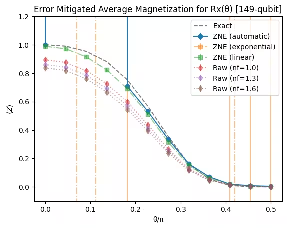
בעוד שהערכים הרועשים (גורם רעש nf=1.0) מראים סטייה גבוהה מהערכים המדויקים, הערכים המופחתים קרובים לערכים המדויקים — דבר המדגים את תועלת טכניקת הפחתת השגיאות מבוססת PEA.
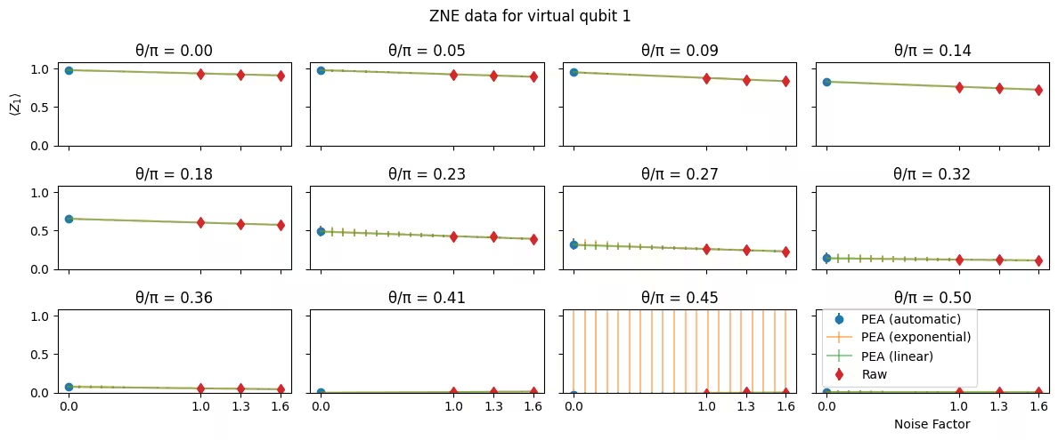
הצגה גרפית של תוצאות אקסטרפולציה עבור קיוביטים בודדים
לבסוף, הקוד הבא יוצר גרף המציג את עקומות האקסטרפולציה עבור ערכים שונים של theta על קיוביט ספציפי.
virtual_qubit = 1
plot_qubit_zne_data(
    pub_result=pub_result,
    angles=parameter_values,
    qubit=virtual_qubit,
    noise_factors=zne_metadata["noise_factors"],
    extrapolator=zne_metadata["extrapolator"],
    extrapolated_noise_factors=zne_metadata["extrapolated_noise_factors"],
)
צעדים הבאים
אם מצאתם את העבודה הזו מעניינת, ייתכן שתתעניינו בחומרים הבאים:
- מדריך המתמקד בשילוב טכניקות הפחתת שגיאות.
- תיעוד מפורט על טכניקות הפחתת השגיאות הזמינות ב-Qiskit.
- שיעורים נוספים המכסים ניסויים בקנה מידה של שירות: Utility II ו-Utility III.