קומפילציה קוונטית קירובית עבור מעגלי אבולוציית זמן

הערכת שימוש: 15 שניות על מעבד Heron (הערה: זוהי הערכה בלבד. זמן הריצה שלך עשוי להשתנות.)

תוצאות למידה

לאחר השלמת מדריך זה, תוכל לצפות להבין את המידע הבא:

כיצד להשתמש ב-AQC-Tensor Qiskit addon לדחיסת מעגלי Trotter עמוקים למעגלי ansatz רדודים
כיצד ליצור ansatz מפרמטר ממעגל Trotter ולבצע אופטימיזציה של הפרמטרים שלו באמצעות שיטות רשת טנזור (MPS)
כיצד להעריך את הנאמנות של מעגל מדוחס מול האבולוציה היעד ולהריץ אותו על חומרה קוונטית

דרישות מוקדמות

מומלץ להכיר את הנושאים הבאים:

רקע

מדריך זה מדגים כיצד ליישם קומפילציה קוונטית קירובית באמצעות רשתות טנזור (AQC-Tensor) עם Qiskit כדי לשפר את ביצועי המעגל הקוונטי. AQC-Tensor דוחסת מעגלי Trotter עמוקים למעגלים רדודים יותר, ידידותיים יותר לחומרה, תוך שמירה על דיוק הסימולציה.

כיצד AQC-Tensor עובד

שקול סימולציה של Hamiltonian $H$ לזמן כולל $t$ באמצעות $k$ צעדי Trotter. מעגל ה-Trotter המלא הוא:

U_{\text{full}} = \left[U_{\text{Trotter}}(t/k)\right]^k

גישה נאיבית משתמשת במעט צעדי Trotter כדי לשמור על עומק מעגל ניתן לניהול, אך זה מכניס שגיאת Trotter משמעותית. AQC-Tensor פותרת את המתח הזה על ידי הפרדת הדיוק מהעומק:

מעגל יעד (דיוק גבוה, עמוק): בנה מעגל Trotter עם צעדים רבים—נניח, $10k$ —לאותו זמן אבולוציה. למעגל זה יש שגיאת Trotter הרבה פחות, אך הוא עמוק מדי לחומרה. מכיוון שהוא מדומה קלאסית בלבד כמצב מכפלת מטריצה (MPS), העומק אינו בעיה.
מעגל ansatz (עומק נמוך, מפרמטר): הגדר מעגל מפרמטר $V(\theta)$ עם אותה מבנה כמו מעגל Trotter של צעד אחד. אתחל אותו כך ש- $V(\theta_{\text{init}}) = U_{\text{Trotter}}(t/k)$ , לאחר מכן בצע אופטימיזציה איטרטיבית של $\theta$ כך ש- $V(\theta)$ ישחזר את מצב היעד בדיוק גבוה בצורה הקרובה ביותר האפשרית.

התוצאה היא מעגל שמשמר את עומק צעד Trotter יחיד אך משיג את הדיוק של רבים, מה שהופך אותו להיתכן לחומרה קוונטית של הדור הקרוב.

מתי להשתמש ב-AQC-Tensor

AQC-Tensor הכי יעיל כאשר:

עומק המעגל עולה על זמני הקוהרנטיות של החומרה. אם סימולציית Trotter דורשת יותר צעדי Trotter ממה שההתקן יכול לתמוך, AQC-Tensor יכול לדחוס את האבולוציה למעגל רדוד יותר.
ההסתבכות נשארת ניתנת לטיפול קלאסי. ההסתבכות הכוללת במצב שעבר אבולוציית זמן תלויה בעיקר בזמן האבולוציה $t$ , לא במספר צעדי Trotter $k$ . פירוש הדבר הוא שמעגל יעד עם $10k$ צעדים בדרך כלל אינו קשה יותר לייצוג כ-MPS מאחד עם $k$ צעדים, כל עוד $t$ קצר מספיק כדי שממדי הקשר יישארו ניתנים לניהול.
קיים ansatz טבעי. מכיוון שה-ansatz משקף את מבנה מעגל Trotter, הוא מספק נקודת התחלה מבוססת פיזיקלית עם פרמטרים ראשוניים מוגדרים היטב, תוך הימנעות מבעיות ההתכנסות שיכולות לפגוע ב-ansatze ווריאציוניים שרירותיים.

גישה זו מנוגדת לדחיסת מעגל גנרית: במקום לנסות לקרב יחידה שרירותית עם פחות שערים, AQC-Tensor שומרת על אותה מבנה שערים ומבצעת אופטימיזציה של הפרמטרים שלה כדי להפחית את שגיאת Trotter. ראה תיעוד AQC-Tensor למידע נוסף.

מדריך זה מנחה אותך דרך תהליך העבודה המלא של הכנת מצב AQC-Tensor: הגדרת Hamiltonian, יצירת מעגלי Trotter, דחיסתם באמצעות אופטימיזציית רשת-טנזור, וביצוע התוצאה על חומרת IBM Quantum®.

דרישות

לפני שתתחיל במדריך זה, ודא שיש לך את הדברים הבאים מותקנים:

Qiskit SDK גרסה 2.0 ואילך, עם תמיכה בויזואליזציה
Qiskit Runtime גרסה 0.22 ואילך (pip install qiskit-ibm-runtime)
הרחבת AQC-Tensor של Qiskit (pip install 'qiskit-addon-aqc-tensor[aer,quimb-jax]')

הגדרה

# Added by doQumentation — required packages for this notebook
!pip install -q matplotlib numpy qiskit qiskit-addon-aqc-tensor qiskit-addon-utils qiskit-ibm-runtime quimb rustworkx scipy

import numpy as np
import quimb.tensor
import datetime
import matplotlib.pyplot as plt

from scipy.linalg import expm
from scipy.optimize import OptimizeResult, minimize

from qiskit.quantum_info import SparsePauliOp, Pauli
from qiskit.transpiler import CouplingMap
from qiskit.transpiler.preset_passmanagers import generate_preset_pass_manager
from qiskit import QuantumCircuit
from qiskit.synthesis import SuzukiTrotter

from qiskit_addon_utils.problem_generators import (
    generate_time_evolution_circuit,
)
from qiskit_addon_aqc_tensor.ansatz_generation import (
    generate_ansatz_from_circuit,
)
from qiskit_addon_aqc_tensor.objective import MaximizeStateFidelity
from qiskit_addon_aqc_tensor.simulation.quimb import QuimbSimulator
from qiskit_addon_aqc_tensor.simulation import tensornetwork_from_circuit
from qiskit_addon_aqc_tensor.simulation import compute_overlap

from qiskit_ibm_runtime import QiskitRuntimeService
from qiskit_ibm_runtime import EstimatorV2 as Estimator
from qiskit_ibm_runtime.fake_provider import FakeKyiv

from rustworkx.visualization import graphviz_draw

דוגמת סימולטור בקנה מידה קטן

חלק זה משתמש במערכת של 10 אתרים כדי להמחיש את תהליך העבודה של AQC-Tensor שלב אחר שלב. אנחנו מדמים את הדינמיקה של שרשרת ספין XXZ בת 10 אתרים, מודל נחקר באופן נרחב לבחינת אינטראקציות ספין ותכונות מגנטיות.

ה-Hamiltonian הוא כדלקמן:

\hat{\mathcal{H}}_{XXZ} = \sum_{i=1}^{L-1} J_{i,(i+1)}\left(X_i X_{(i+1)}+Y_i Y_{(i+1)}+ 2\cdot Z_i Z_{(i+1)} \right) \, ,

כאשר $J_{i,(i+1)}$ הוא מקדם אקראי לקצה $(i, i+1)$ ו- $L=10$ .

שלב 1: מיפוי קלטים קלאסיים לבעיה קוונטית

בשלב זה, אנחנו:

מגדירים את ה-Hamiltonian, ה-observable והמצב הראשוני.
מחשבים את ערך הציפייה המדויק קלאסית להשוואה מאוחרת יותר.
מייצרים מעגל Trotter בדיוק גבוה (יעד ה-AQC) ודוחסים אותו ל-ansatz בעומק נמוך באמצעות AQC-Tensor.

הגדרת ה-Hamiltonian, ה-observable והמצב הראשוני

# L is the number of sites in the 1D spin chain
L = 10

# Generate the coupling map
edge_list = [(i - 1, i) for i in range(1, L)]
even_edges = edge_list[::2]
odd_edges = edge_list[1::2]
coupling_map = CouplingMap(edge_list)

# Generate random coefficients for our XXZ Hamiltonian
np.random.seed(0)
Js = np.random.rand(L - 1) + 0.5 * np.ones(L - 1)
hamiltonian = SparsePauliOp(Pauli("I" * L))
for i, edge in enumerate(even_edges + odd_edges):
    hamiltonian += SparsePauliOp.from_sparse_list(
        [
            ("XX", (edge), Js[i] / 2),
            ("YY", (edge), Js[i] / 2),
            ("ZZ", (edge), Js[i]),
        ],
        num_qubits=L,
    )

# Generate a ZZ observable between the two middle qubits
observable = SparsePauliOp.from_sparse_list(
    [("ZZ", (L // 2 - 1, L // 2), 1.0)], num_qubits=L
)

# Generate an initial Néel state |1010101010⟩
initial_state_circuit = QuantumCircuit(L)
for i in range(L):
    if i % 2:
        initial_state_circuit.x(i)

print("Hamiltonian:", hamiltonian)
print("Observable:", observable)
graphviz_draw(coupling_map.graph, method="circo")

Hamiltonian: SparsePauliOp(['IIIIIIIIII', 'IIIIIIIIXX', 'IIIIIIIIYY', 'IIIIIIIIZZ', 'IIIIIIXXII', 'IIIIIIYYII', 'IIIIIIZZII', 'IIIIXXIIII', 'IIIIYYIIII', 'IIIIZZIIII', 'IIXXIIIIII', 'IIYYIIIIII', 'IIZZIIIIII', 'XXIIIIIIII', 'YYIIIIIIII', 'ZZIIIIIIII', 'IIIIIIIXXI', 'IIIIIIIYYI', 'IIIIIIIZZI', 'IIIIIXXIII', 'IIIIIYYIII', 'IIIIIZZIII', 'IIIXXIIIII', 'IIIYYIIIII', 'IIIZZIIIII', 'IXXIIIIIII', 'IYYIIIIIII', 'IZZIIIIIII'],
              coeffs=[1.        +0.j, 0.52440675+0.j, 0.52440675+0.j, 1.0488135 +0.j,
 0.60759468+0.j, 0.60759468+0.j, 1.21518937+0.j, 0.55138169+0.j,
 0.55138169+0.j, 1.10276338+0.j, 0.52244159+0.j, 0.52244159+0.j,
 1.04488318+0.j, 0.4618274 +0.j, 0.4618274 +0.j, 0.9236548 +0.j,
 0.57294706+0.j, 0.57294706+0.j, 1.14589411+0.j, 0.46879361+0.j,
 0.46879361+0.j, 0.93758721+0.j, 0.6958865 +0.j, 0.6958865 +0.j,
 1.391773  +0.j, 0.73183138+0.j, 0.73183138+0.j, 1.46366276+0.j])
Observable: SparsePauliOp(['IIIIZZIIII'],
              coeffs=[1.+0.j])

Output of the previous code cell

חישוב ערך הציפייה המדויק

עבור מערכת בגודל זה, ניתן לחשב את ערך הציפייה המדויק של אבולוציית הזמן ישירות באמצעות חזקת מטריצה. זה ישמש כאמת הקרקע שלנו להערכת הדיוק של מעגל ה-AQC.

aqc_evolution_time = 0.2

# Each baseline Trotter step covers dt = aqc_evolution_time / 3
# The subsequent (uncompressed) step covers 1 additional dt
subsequent_evolution_time = aqc_evolution_time / 3
total_evolution_time = aqc_evolution_time + subsequent_evolution_time

# Compute exact expectation value via matrix exponentiation
H_matrix = hamiltonian.to_matrix()
U_exact = expm(-1j * H_matrix * total_evolution_time)

# Build the initial state vector (Néel state)
initial_state_vec = np.zeros(2**L)
state_idx = sum(2**i for i in range(L) if i % 2)
initial_state_vec[state_idx] = 1.0

# Evolve and compute expectation value
evolved_state = U_exact @ initial_state_vec
obs_matrix = observable.to_matrix()
exact_expval = (evolved_state.conj() @ obs_matrix @ evolved_state).real

print(f"AQC evolution time: {aqc_evolution_time}")
print(f"Subsequent evolution time: {subsequent_evolution_time:.6f}")
print(f"Total evolution time: {total_evolution_time:.6f}")
print(f"Exact expectation value: {exact_expval:.6f}")

AQC evolution time: 0.2
Subsequent evolution time: 0.066667
Total evolution time: 0.266667
Exact expectation value: -0.700899

יצירת מעגל יעד ה-AQC

כעת אנחנו בונים את מעגל ה-Trotter שישמש כיעד ה-AQC. מעגל זה משתמש בצעדי Trotter רבים (32) לדיוק גבוה. מכיוון שהוא ידומה קלאסית בלבד כ-MPS—ולא יבוצע על חומרה—העומק הגדול אינו בעיה.

aqc_target_num_trotter_steps = 32

aqc_target_circuit = initial_state_circuit.copy()
aqc_target_circuit.compose(
    generate_time_evolution_circuit(
        hamiltonian,
        synthesis=SuzukiTrotter(reps=aqc_target_num_trotter_steps),
        time=aqc_evolution_time,
    ),
    inplace=True,
)

יצירת ansatz, פרמטרים ראשוניים, מעגל עוקב ומעגל בסיס

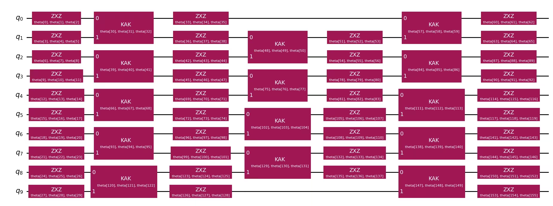
בשלב הבא, אנחנו בונים מעגל "טוב" עם אותו זמן אבולוציה כמו יעד ה-AQC אך עם הרבה פחות צעדי Trotter (רק אחד). אנחנו מעבירים מעגל זה ל-generate_ansatz_from_circuit, שמחזיר:

מעגל ansatz כללי ומפרמטר עם אותה קישוריות של שני-qubit.
פרמטרים ראשוניים שמשחזרים את מעגל הקלט כאשר מחוברים ל-ansatz.

אנחנו גם בונים:

מעגל עוקב עם צעד Trotter אחד שיצורף (לא מדוחס) לאחר החלק המותאם של AQC, בעקבות הגישה ב-מדריך מצב התחלתי של AQC-Tensor.
מעגל Trotter בסיס המשתמש בארבעה צעדי Trotter לאורך זמן האבולוציה המלא (aqc_evolution_time + subsequent_evolution_time). זה ישמש כהשוואה: הוא מייצג מה שהיית מריץ על חומרה ללא AQC. מעגל ה-ansatz של AQC (3 צעדים מדוחסים + 1 לא מדוחס) משיג דיוק טוב יותר בעומק נמוך יותר.

aqc_ansatz_num_trotter_steps = 1

aqc_good_circuit = initial_state_circuit.copy()
aqc_good_circuit.compose(
    generate_time_evolution_circuit(
        hamiltonian,
        synthesis=SuzukiTrotter(reps=aqc_ansatz_num_trotter_steps),
        time=aqc_evolution_time,
    ),
    inplace=True,
)

aqc_ansatz, aqc_initial_parameters = generate_ansatz_from_circuit(
    aqc_good_circuit
)

# Subsequent circuit: 1 non-compressed Trotter step appended after AQC
subsequent_num_trotter_steps = 1
subsequent_circuit = generate_time_evolution_circuit(
    hamiltonian,
    synthesis=SuzukiTrotter(reps=subsequent_num_trotter_steps),
    time=subsequent_evolution_time,
)

# Baseline Trotter circuit: 4 Trotter steps over total evolution time, no AQC
baseline_num_trotter_steps = 4
baseline_circuit = initial_state_circuit.copy()
baseline_circuit.compose(
    generate_time_evolution_circuit(
        hamiltonian,
        synthesis=SuzukiTrotter(reps=baseline_num_trotter_steps),
        time=total_evolution_time,
    ),
    inplace=True,
)

print(
    f"Target circuit:      depth {aqc_target_circuit.depth(lambda x: x.operation.num_qubits == 2)}"
)
print(
    f"Baseline circuit:    depth {baseline_circuit.depth(lambda x: x.operation.num_qubits == 2)} ({baseline_num_trotter_steps} Trotter steps, time={total_evolution_time:.4f})"
)
print(
    f"Subsequent circuit:  depth {subsequent_circuit.depth(lambda x: x.operation.num_qubits == 2)} ({subsequent_num_trotter_steps} Trotter step, time={subsequent_evolution_time:.4f})"
)
print(
    f"Ansatz circuit:      depth {aqc_ansatz.depth(lambda x: x.operation.num_qubits == 2)}, with {len(aqc_initial_parameters)} parameters"
)
aqc_ansatz.draw("mpl", fold=-1)

Target circuit:      depth 384
Baseline circuit:    depth 48 (4 Trotter steps, time=0.2667)
Subsequent circuit:  depth 12 (1 Trotter step, time=0.0667)
Ansatz circuit:      depth 3, with 156 parameters

Output of the previous code cell

הגדרת סימולציית רשת טנזור ובניית MPS היעד

אנחנו משתמשים בסימולטור מעגל מצב מכפלת מטריצה (MPS) של quimb, כאשר JAX מספק גזירה אוטומטית לאופטימיזציה מבוססת-גרדיאנט. לאחר מכן אנחנו בונים ייצוג MPS של המצב היעד ומעריכים את הנאמנות ההתחלתית בין ה-ansatz הראשוני לבין היעד. מכיוון שזו דוגמה קטנה יחסית, הנאמנות ההתחלתית מתחילה גבוהה למדי.

simulator_settings = QuimbSimulator(
    quimb.tensor.CircuitMPS, autodiff_backend="jax"
)

aqc_target_mps = tensornetwork_from_circuit(
    aqc_target_circuit, simulator_settings
)
print("Target MPS maximum bond dimension:", aqc_target_mps.psi.max_bond())

good_mps = tensornetwork_from_circuit(aqc_good_circuit, simulator_settings)
starting_fidelity = abs(compute_overlap(good_mps, aqc_target_mps)) ** 2
print(f"Starting fidelity: {starting_fidelity:.6f}")

Target MPS maximum bond dimension: 5
Starting fidelity: 0.998246

אופטימיזציה של פרמטרי ה-ansatz

אנחנו ממזערים את פונקציית העלות MaximizeStateFidelity באמצעות אופטימייזר L-BFGS-B. האופטימייזר מתאים באופן איטרטיבי את פרמטרי ה-ansatz כדי למקסם את הנאמנות בין מעגל ה-ansatz לבין MPS היעד.

aqc_stopping_fidelity = 1
aqc_max_iterations = 500

stopping_point = 1.0 - aqc_stopping_fidelity
objective = MaximizeStateFidelity(
    aqc_target_mps, aqc_ansatz, simulator_settings
)

def callback(intermediate_result: OptimizeResult):
    fidelity = 1 - intermediate_result.fun
    print(
        f"{datetime.datetime.now()} Intermediate result: Fidelity {fidelity:.8f}"
    )
    if intermediate_result.fun < stopping_point:
        raise StopIteration

result = minimize(
    objective,
    aqc_initial_parameters,
    method="L-BFGS-B",
    jac=True,
    options={"maxiter": aqc_max_iterations},
    callback=callback,
)
if result.status not in (0, 1, 99):
    raise RuntimeError(
        f"Optimization failed: {result.message} (status={result.status})"
    )

print(f"Done after {result.nit} iterations.")
aqc_final_parameters = result.x

2026-05-18 13:14:49.731596 Intermediate result: Fidelity 0.99952882
2026-05-18 13:14:49.734425 Intermediate result: Fidelity 0.99958531
2026-05-18 13:14:49.737101 Intermediate result: Fidelity 0.99960093
2026-05-18 13:14:49.739813 Intermediate result: Fidelity 0.99961046
2026-05-18 13:14:49.742969 Intermediate result: Fidelity 0.99962560
2026-05-18 13:14:49.745916 Intermediate result: Fidelity 0.99964395
2026-05-18 13:14:49.748615 Intermediate result: Fidelity 0.99968150
2026-05-18 13:14:49.753684 Intermediate result: Fidelity 0.99970569
2026-05-18 13:14:49.756208 Intermediate result: Fidelity 0.99973788
2026-05-18 13:14:49.759067 Intermediate result: Fidelity 0.99975385
2026-05-18 13:14:49.762321 Intermediate result: Fidelity 0.99976458
2026-05-18 13:14:49.765526 Intermediate result: Fidelity 0.99977661
2026-05-18 13:14:49.768496 Intermediate result: Fidelity 0.99978663
2026-05-18 13:14:49.771278 Intermediate result: Fidelity 0.99980236
2026-05-18 13:14:49.773735 Intermediate result: Fidelity 0.99981607
2026-05-18 13:14:49.776339 Intermediate result: Fidelity 0.99982811
2026-05-18 13:14:49.779177 Intermediate result: Fidelity 0.99985827
2026-05-18 13:14:49.782243 Intermediate result: Fidelity 0.99988354
2026-05-18 13:14:49.784904 Intermediate result: Fidelity 0.99991608
2026-05-18 13:14:49.787737 Intermediate result: Fidelity 0.99993336
2026-05-18 13:14:49.790414 Intermediate result: Fidelity 0.99993956
2026-05-18 13:14:49.793029 Intermediate result: Fidelity 0.99994421
2026-05-18 13:14:49.795585 Intermediate result: Fidelity 0.99994743
2026-05-18 13:14:49.835045 Intermediate result: Fidelity 0.99994791
2026-05-18 13:14:49.839786 Intermediate result: Fidelity 0.99994803
2026-05-18 13:14:49.842403 Intermediate result: Fidelity 0.99994898
2026-05-18 13:14:49.873779 Intermediate result: Fidelity 0.99994898
Done after 27 iterations.

הרכבת מעגל AQC הסופי

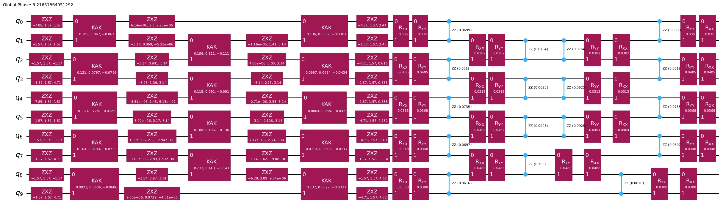
עם הפרמטרים המותאמים בידינו, אנחנו מחברים אותם ל-ansatz ולאחר מכן מצרפים את צעד ה-Trotter העוקב (הלא מדוחס). למעגל המתקבל יש את עומק צעד Trotter מדוחס יחיד בתוספת צעד אחד לא מדוחס, אך החלק המדוחס מקרב את הדיוק של 32 צעדי Trotter.

aqc_final_circuit = aqc_ansatz.assign_parameters(aqc_final_parameters)
aqc_final_circuit.compose(subsequent_circuit, inplace=True)
aqc_final_circuit.draw("mpl", fold=-1)

Output of the previous code cell

שלב 2: אופטימיזציה של הבעיה לביצוע חומרה קוונטית

לדוגמה בקנה מידה קטן זו, אנחנו משתמשים ב-backend מדומה (FakeKyiv) לסימולציה של ביצוע חומרה מקומית. אנחנו מבצעים טרנספילציה של מעגל ה-AQC המותאם (aqc_final_circuit) ושל מעגל ה-Trotter הבסיסי (baseline_circuit, ארבעה צעדי Trotter לאורך זמן האבולוציה המלא, ללא AQC) ל-ISA של ה-backend (ארכיטקטורת קבוצת ההוראות), עם optimization_level=3 להפחתת עומק המעגל עוד יותר.

backend = FakeKyiv()

pass_manager = generate_preset_pass_manager(
    backend=backend, optimization_level=3
)

# Transpile the AQC-optimized circuit (compressed + subsequent step)
isa_circuit = pass_manager.run(aqc_final_circuit)
isa_observable = observable.apply_layout(isa_circuit.layout)
print(
    "AQC circuit depth:",
    isa_circuit.depth(lambda x: x.operation.num_qubits == 2),
)

# Transpile the baseline Trotter circuit (no AQC optimization)
isa_baseline_circuit = pass_manager.run(baseline_circuit)
isa_baseline_observable = observable.apply_layout(isa_baseline_circuit.layout)
print(
    "Baseline Trotter circuit depth:",
    isa_baseline_circuit.depth(lambda x: x.operation.num_qubits == 2),
)

AQC circuit depth: 15
Baseline Trotter circuit depth: 27

שלב 3: ביצוע באמצעות primitives של Qiskit

אנחנו משתמשים ב-primitive EstimatorV2 עם ה-backend המדומה להרצת גם מעגל ה-AQC המותאם וגם מעגל ה-Trotter הבסיסי, תוך מדידת ה-observable ZZ עבור כל אחד.

estimator = Estimator(backend)

# Run both circuits
aqc_result = estimator.run([(isa_circuit, isa_observable)]).result()
baseline_result = estimator.run(
    [(isa_baseline_circuit, isa_baseline_observable)]
).result()

שלב 4: עיבוד לאחר ביצוע והחזרת תוצאה בפורמט קלאסי רצוי

אנחנו מחלצים את ערכי הציפייה משתי ההרצות ומשווים אותם לתוצאה המדויקת. מעגל ה-Trotter הבסיסי מראה מה היינו מקבלים ללא AQC באותו עומק מעגל, בעוד מעגל ה-AQC מדגים את השיפור מאופטימיזציית רשת-טנזור.

aqc_expval = aqc_result[0].data.evs.tolist()
baseline_expval = baseline_result[0].data.evs.tolist()

print(f"Exact:              {exact_expval:.4f}")
print(
    f"Baseline Trotter:   {baseline_expval:.4f}, |\u0394| = {np.abs(exact_expval - baseline_expval):.4f}  (depth {isa_baseline_circuit.depth(lambda x: x.operation.num_qubits == 2)}, {baseline_num_trotter_steps} steps)"
)
print(
    f"AQC (3+1):          {aqc_expval:.4f}, |\u0394| = {np.abs(exact_expval - aqc_expval):.4f}  (depth {isa_circuit.depth(lambda x: x.operation.num_qubits == 2)}, compressed+subsequent)"
)

Exact:              -0.7009
Baseline Trotter:   -0.5400, |Δ| = 0.1609  (depth 27, 4 steps)
AQC (3+1):          -0.5728, |Δ| = 0.1281  (depth 15, compressed+subsequent)

plt.style.use("seaborn-v0_8")

labels = [
    f"Baseline Trotter\n({baseline_num_trotter_steps} steps, depth {isa_baseline_circuit.depth(lambda x: x.operation.num_qubits == 2)})",
    f"AQC (3+1)\n(depth {isa_circuit.depth(lambda x: x.operation.num_qubits == 2)})",
]
values = [baseline_expval, aqc_expval]
colors = ["tab:orange", "tab:blue"]

plt.figure(figsize=(8, 5))
bars = plt.bar(labels, values, color=colors, width=0.5)
plt.axhline(
    y=exact_expval,
    color="tab:green",
    linestyle="--",
    linewidth=2,
    label=f"Exact ({exact_expval:.4f})",
)
plt.ylabel("Expected Value")
plt.title(
    "AQC-Tensor (3 compressed + 1 uncompressed) vs Baseline Trotter (10-site XXZ)"
)
plt.legend()
for bar in bars:
    y_val = bar.get_height()
    plt.text(
        bar.get_x() + bar.get_width() / 2.0,
        y_val,
        f"{y_val:.4f}",
        ha="center",
        va="bottom" if y_val >= 0 else "top",
    )
plt.axhline(y=0, color="black", linewidth=0.3)
plt.tight_layout()
plt.show()

Output of the previous code cell

דוגמת חומרה בקנה מידה גדול

כעת אנחנו מגדילים את קנה המידה למודל XXZ בן 50 אתרים כדי להדגים את AQC-Tensor על גודל בעיה ריאליסטי יותר. תהליך העבודה זהה לדוגמה בקנה מידה הקטן: אנחנו דוחסים שלושה צעדי Trotter דרך AQC ומצרפים צעד אחד לא מדוחס.

עבור מערכת בגודל זה, חזקת מטריצה אינה ניתנת לביצוע ( $2^{50}$ ממדים), לכן אנחנו מחשבים את ערך הציפייה הייחוסי ישירות מ-MPS בדיוק גבוה שעבר אבולוציה לאורך הזמן המלא.

שלבים 1–4 משולבים

# -------------------------Step 1-------------------------

# Define the 50-site spin chain
L = 50
edge_list = [(i - 1, i) for i in range(1, L)]
even_edges = edge_list[::2]
odd_edges = edge_list[1::2]
coupling_map = CouplingMap(edge_list)

# Random XXZ Hamiltonian
np.random.seed(0)
Js = np.random.rand(L - 1) + 0.5 * np.ones(L - 1)
hamiltonian = SparsePauliOp(Pauli("I" * L))
for i, edge in enumerate(even_edges + odd_edges):
    hamiltonian += SparsePauliOp.from_sparse_list(
        [
            ("XX", (edge), Js[i] / 2),
            ("YY", (edge), Js[i] / 2),
            ("ZZ", (edge), Js[i]),
        ],
        num_qubits=L,
    )

observable = SparsePauliOp.from_sparse_list(
    [("ZZ", (L // 2 - 1, L // 2), 1.0)], num_qubits=L
)

# Initial Néel state
initial_state_circuit = QuantumCircuit(L)
for i in range(L):
    if i % 2:
        initial_state_circuit.x(i)

# Time parameters
aqc_evolution_time = 0.2
subsequent_evolution_time = aqc_evolution_time / 3
total_evolution_time = aqc_evolution_time + subsequent_evolution_time

# AQC target circuit (high-accuracy, 32 Trotter steps for AQC portion)
aqc_target_num_trotter_steps = 32

aqc_target_circuit = initial_state_circuit.copy()
aqc_target_circuit.compose(
    generate_time_evolution_circuit(
        hamiltonian,
        synthesis=SuzukiTrotter(reps=aqc_target_num_trotter_steps),
        time=aqc_evolution_time,
    ),
    inplace=True,
)

# Generate ansatz from 1-step Trotter circuit
aqc_good_circuit = initial_state_circuit.copy()
aqc_good_circuit.compose(
    generate_time_evolution_circuit(
        hamiltonian,
        synthesis=SuzukiTrotter(reps=1),
        time=aqc_evolution_time,
    ),
    inplace=True,
)

aqc_ansatz, aqc_initial_parameters = generate_ansatz_from_circuit(
    aqc_good_circuit
)

# Subsequent circuit: 1 non-compressed Trotter step
subsequent_circuit = generate_time_evolution_circuit(
    hamiltonian,
    synthesis=SuzukiTrotter(reps=1),
    time=subsequent_evolution_time,
)

# Baseline Trotter circuit: 4 Trotter steps over total evolution time, no AQC
baseline_num_trotter_steps = 4
baseline_circuit = initial_state_circuit.copy()
baseline_circuit.compose(
    generate_time_evolution_circuit(
        hamiltonian,
        synthesis=SuzukiTrotter(reps=baseline_num_trotter_steps),
        time=total_evolution_time,
    ),
    inplace=True,
)
print(
    f"Target circuit:  depth {aqc_target_circuit.depth(lambda x: x.operation.num_qubits == 2)}"
)
print(
    f"Ansatz circuit:  depth {aqc_ansatz.depth(lambda x: x.operation.num_qubits == 2)}, with {len(aqc_initial_parameters)} parameters"
)
print(
    f"Subsequent circuit: depth {subsequent_circuit.depth(lambda x: x.operation.num_qubits == 2)}"
)
print(
    f"Baseline circuit:   depth {baseline_circuit.depth(lambda x: x.operation.num_qubits == 2)} ({baseline_num_trotter_steps} steps, time={total_evolution_time:.4f})"
)

# Build target MPS and compute reference expectation value
simulator_settings = QuimbSimulator(
    quimb.tensor.CircuitMPS, autodiff_backend="jax"
)
aqc_target_mps = tensornetwork_from_circuit(
    aqc_target_circuit, simulator_settings
)
print("Target MPS maximum bond dimension:", aqc_target_mps.psi.max_bond())

# For the reference expectation value, we need the full evolution (AQC + subsequent)
# Build a high-accuracy full circuit for MPS reference
full_target_circuit = initial_state_circuit.copy()
full_target_circuit.compose(
    generate_time_evolution_circuit(
        hamiltonian,
        synthesis=SuzukiTrotter(reps=aqc_target_num_trotter_steps),
        time=total_evolution_time,
    ),
    inplace=True,
)
full_target_mps = tensornetwork_from_circuit(
    full_target_circuit, simulator_settings
)
exact_expval = full_target_mps.local_expectation(
    quimb.pauli("Z") & quimb.pauli("Z"), (L // 2 - 1, L // 2)
).real.item()
print(f"Reference expectation value (from MPS): {exact_expval:.6f}")

# Optimize ansatz parameters
objective = MaximizeStateFidelity(
    aqc_target_mps, aqc_ansatz, simulator_settings
)

def callback(intermediate_result: OptimizeResult):
    fidelity = 1 - intermediate_result.fun
    print(
        f"{datetime.datetime.now()} Intermediate result: Fidelity {fidelity:.8f}"
    )

result = minimize(
    objective,
    aqc_initial_parameters,
    method="L-BFGS-B",
    jac=True,
    options={"maxiter": 500},
    callback=callback,
)
if result.status not in (0, 1, 99):
    raise RuntimeError(
        f"Optimization failed: {result.message} (status={result.status})"
    )
print(f"Done after {result.nit} iterations.")

# Assemble the final AQC circuit: optimized ansatz + subsequent Trotter step
aqc_final_circuit = aqc_ansatz.assign_parameters(result.x)
aqc_final_circuit.compose(subsequent_circuit, inplace=True)

# -------------------------Step 2-------------------------

service = QiskitRuntimeService()
backend = service.least_busy(min_num_qubits=127)
print(backend)

pass_manager = generate_preset_pass_manager(
    backend=backend, optimization_level=3
)
isa_circuit = pass_manager.run(aqc_final_circuit)
isa_observable = observable.apply_layout(isa_circuit.layout)
print(
    "AQC circuit depth:",
    isa_circuit.depth(lambda x: x.operation.num_qubits == 2),
)

# Also transpile the baseline Trotter circuit (4 Trotter steps, no AQC)
isa_baseline_circuit = pass_manager.run(baseline_circuit)
isa_baseline_observable = observable.apply_layout(isa_baseline_circuit.layout)
print(
    "Baseline Trotter circuit depth:",
    isa_baseline_circuit.depth(lambda x: x.operation.num_qubits == 2),
)

# -------------------------Step 3-------------------------

# Submit both circuits in a single job
estimator = Estimator(backend)
estimator.options.environment.job_tags = ["TUT_AQCTE"]

job = estimator.run(
    [
        (isa_circuit, isa_observable),
        (isa_baseline_circuit, isa_baseline_observable),
    ]
)
print("Job ID:", job.job_id())

Target circuit:  depth 385
Ansatz circuit:  depth 7, with 816 parameters
Subsequent circuit: depth 12
Baseline circuit:   depth 49 (4 steps, time=0.2667)
Target MPS maximum bond dimension: 5
Reference expectation value (from MPS): -0.738669
2026-05-18 13:02:11.219150 Intermediate result: Fidelity 0.99795732
2026-05-18 13:02:11.232256 Intermediate result: Fidelity 0.99822481
2026-05-18 13:02:11.245160 Intermediate result: Fidelity 0.99829520
2026-05-18 13:02:11.257765 Intermediate result: Fidelity 0.99832379
2026-05-18 13:02:11.270280 Intermediate result: Fidelity 0.99836416
2026-05-18 13:02:11.284116 Intermediate result: Fidelity 0.99840073
2026-05-18 13:02:11.296856 Intermediate result: Fidelity 0.99846863
2026-05-18 13:02:11.309602 Intermediate result: Fidelity 0.99865244
2026-05-18 13:02:11.322012 Intermediate result: Fidelity 0.99872665
2026-05-18 13:02:11.334195 Intermediate result: Fidelity 0.99892335
2026-05-18 13:02:11.346570 Intermediate result: Fidelity 0.99901045
2026-05-18 13:02:11.359202 Intermediate result: Fidelity 0.99907181
2026-05-18 13:02:11.371511 Intermediate result: Fidelity 0.99911125
2026-05-18 13:02:11.383870 Intermediate result: Fidelity 0.99918585
2026-05-18 13:02:11.396184 Intermediate result: Fidelity 0.99921504
2026-05-18 13:02:11.408543 Intermediate result: Fidelity 0.99924936
2026-05-18 13:02:11.422557 Intermediate result: Fidelity 0.99929226
2026-05-18 13:02:11.436275 Intermediate result: Fidelity 0.99933099
2026-05-18 13:02:11.449511 Intermediate result: Fidelity 0.99935792
2026-05-18 13:02:11.462093 Intermediate result: Fidelity 0.99937925
2026-05-18 13:02:11.475783 Intermediate result: Fidelity 0.99940690
2026-05-18 13:02:11.490254 Intermediate result: Fidelity 0.99944409
2026-05-18 13:02:11.503292 Intermediate result: Fidelity 0.99946840
2026-05-18 13:02:11.516064 Intermediate result: Fidelity 0.99949378
2026-05-18 13:02:11.532861 Intermediate result: Fidelity 0.99951380
2026-05-18 13:02:11.546182 Intermediate result: Fidelity 0.99955313
2026-05-18 13:02:11.559168 Intermediate result: Fidelity 0.99955707
2026-05-18 13:02:11.571753 Intermediate result: Fidelity 0.99959306
2026-05-18 13:02:11.584257 Intermediate result: Fidelity 0.99960486
2026-05-18 13:02:11.597610 Intermediate result: Fidelity 0.99961714
2026-05-18 13:02:11.610106 Intermediate result: Fidelity 0.99962953
2026-05-18 13:02:11.622515 Intermediate result: Fidelity 0.99963525
2026-05-18 13:02:11.635543 Intermediate result: Fidelity 0.99964658
2026-05-18 13:02:11.649044 Intermediate result: Fidelity 0.99965027
2026-05-18 13:02:11.664148 Intermediate result: Fidelity 0.99965802
2026-05-18 13:02:11.678033 Intermediate result: Fidelity 0.99966731
2026-05-18 13:02:11.692714 Intermediate result: Fidelity 0.99967780
2026-05-18 13:02:11.706753 Intermediate result: Fidelity 0.99968567
2026-05-18 13:02:11.720780 Intermediate result: Fidelity 0.99969139
2026-05-18 13:02:11.733471 Intermediate result: Fidelity 0.99969628
2026-05-18 13:02:11.745998 Intermediate result: Fidelity 0.99970331
2026-05-18 13:02:11.758424 Intermediate result: Fidelity 0.99970796
2026-05-18 13:02:11.771986 Intermediate result: Fidelity 0.99971165
2026-05-18 13:02:11.785841 Intermediate result: Fidelity 0.99971892
2026-05-18 13:02:11.799105 Intermediate result: Fidelity 0.99972226
2026-05-18 13:02:11.811623 Intermediate result: Fidelity 0.99972441
2026-05-18 13:02:11.824114 Intermediate result: Fidelity 0.99972679
2026-05-18 13:02:11.837179 Intermediate result: Fidelity 0.99972965
2026-05-18 13:02:12.345479 Intermediate result: Fidelity 0.99972965
Done after 49 iterations.
<IBMBackend('ibm_pittsburgh')>
AQC circuit depth: 71
Baseline Trotter circuit depth: 111
Job ID: d85kc6o0bvlc73d5nhn0

# -------------------------Step 4-------------------------

hw_results = job.result()
aqc_expval = hw_results[0].data.evs.tolist()
baseline_expval = hw_results[1].data.evs.tolist()

print(f"Exact (MPS):        {exact_expval:.4f}")
print(
    f"Baseline Trotter:   {baseline_expval:.4f}, |\u0394| = {np.abs(exact_expval - baseline_expval):.4f}"
)
print(
    f"AQC (3+1):          {aqc_expval:.4f}, |\u0394| = {np.abs(exact_expval - aqc_expval):.4f}"
)

labels = [
    f"Baseline Trotter\n({baseline_num_trotter_steps} steps, depth {isa_baseline_circuit.depth(lambda x: x.operation.num_qubits == 2)})",
    f"AQC (3+1)\n(depth {isa_circuit.depth(lambda x: x.operation.num_qubits == 2)})",
]
values = [baseline_expval, aqc_expval]
colors = ["tab:orange", "tab:blue"]

plt.figure(figsize=(8, 5))
bars = plt.bar(labels, values, color=colors, width=0.5)
plt.axhline(
    y=exact_expval,
    color="tab:green",
    linestyle="--",
    linewidth=2,
    label=f"Exact ({exact_expval:.4f})",
)
plt.ylabel("Expected Value")
plt.title(
    "AQC-Tensor (3 compressed + 1 uncompressed) vs Baseline Trotter (50-site XXZ)"
)
plt.legend()
for bar in bars:
    y_val = bar.get_height()
    plt.text(
        bar.get_x() + bar.get_width() / 2.0,
        y_val,
        f"{y_val:.4f}",
        ha="center",
        va="bottom" if y_val >= 0 else "top",
    )
plt.axhline(y=0, color="black", linewidth=0.3)
plt.tight_layout()
plt.show()

Exact (MPS):        -0.7387
Baseline Trotter:   -0.5955, |Δ| = 0.1432
AQC (3+1):          -0.6734, |Δ| = 0.0653

Output of the previous code cell

הצעדים הבאים

המלצות

אם מצאת עבודה זו מעניינת, ייתכן שתתעניין בחומר הבא:

תיעוד AQC-Tensor addon — כולל את הטכניקה הקשורה AQC יחידתי, המבצעת אופטימיזציה של מעגלים מפרמטרים לקירוב אופרטור יחידתי יעד במקום מצב מוכן
טכניקות הפחתה ודיכוי שגיאות
שלב טכניקות הפחתת שגיאות

תוצאות למידה​

דרישות מוקדמות​

רקע​

כיצד AQC-Tensor עובד​

מתי להשתמש ב-AQC-Tensor​

דרישות​

הגדרה​

דוגמת סימולטור בקנה מידה קטן​

שלב 1: מיפוי קלטים קלאסיים לבעיה קוונטית​

הגדרת ה-Hamiltonian, ה-observable והמצב הראשוני​

חישוב ערך הציפייה המדויק​

יצירת מעגל יעד ה-AQC​

יצירת ansatz, פרמטרים ראשוניים, מעגל עוקב ומעגל בסיס​

הגדרת סימולציית רשת טנזור ובניית MPS היעד​

אופטימיזציה של פרמטרי ה-ansatz​

הרכבת מעגל AQC הסופי​

שלב 2: אופטימיזציה של הבעיה לביצוע חומרה קוונטית​

שלב 3: ביצוע באמצעות primitives של Qiskit​

שלב 4: עיבוד לאחר ביצוע והחזרת תוצאה בפורמט קלאסי רצוי​

דוגמת חומרה בקנה מידה גדול​

שלבים 1–4 משולבים​

הצעדים הבאים​

תוצאות למידה

דרישות מוקדמות

רקע

כיצד AQC-Tensor עובד

מתי להשתמש ב-AQC-Tensor

דרישות

הגדרה

דוגמת סימולטור בקנה מידה קטן

שלב 1: מיפוי קלטים קלאסיים לבעיה קוונטית

הגדרת ה-Hamiltonian, ה-observable והמצב הראשוני

חישוב ערך הציפייה המדויק

יצירת מעגל יעד ה-AQC

יצירת ansatz, פרמטרים ראשוניים, מעגל עוקב ומעגל בסיס

הגדרת סימולציית רשת טנזור ובניית MPS היעד

אופטימיזציה של פרמטרי ה-ansatz

הרכבת מעגל AQC הסופי

שלב 2: אופטימיזציה של הבעיה לביצוע חומרה קוונטית

שלב 3: ביצוע באמצעות primitives של Qiskit

שלב 4: עיבוד לאחר ביצוע והחזרת תוצאה בפורמט קלאסי רצוי

דוגמת חומרה בקנה מידה גדול

שלבים 1–4 משולבים

הצעדים הבאים