אלכסון קוונטי קרילוב של המילטוניאנים במבנה רשת

הערכת שימוש: 20 דקות על Heron r2 (הערה: זוהי הערכה בלבד. זמן הריצה שלך עשוי להשתנות.)

# Added by doQumentation — required packages for this notebook
!pip install -q matplotlib numpy qiskit qiskit-ibm-runtime scipy sympy

# This cell is hidden from users – it disables some lint rules
# ruff: noqa: E402 E722 F601

רקע

מדריך זה מדגים כיצד ליישם את אלגוריתם האלכסון הקוונטי קרילוב (KQD) בהקשר של תבניות Qiskit. תחילה תלמד על התיאוריה מאחורי האלגוריתם ולאחר מכן תראה הדגמה של ביצועו על QPU.

בתחומים שונים, אנחנו מעוניינים ללמוד תכונות של מצב היסוד של מערכות קוונטיות. דוגמאות כוללות הבנת האופי הבסיסי של חלקיקים וכוחות, חיזוי והבנת התנהגות של חומרים מורכבים והבנת אינטראקציות וריאקציות ביוכימיות. בשל הצמיחה האקספוננציאלית של מרחב הילברט והקורלציה הנוצרת במערכות שזורות, אלגוריתמים קלאסיים מתקשים לפתור בעיה זו עבור מערכות קוונטיות בגודל הולך וגדל. בקצה אחד של הספקטרום נמצאת הגישה הקיימת שמנצלת את החומרה הקוונטית המתמקדת בשיטות קוונטיות וריאציוניות (לדוגמה, variational quantum eigensolver). טכניקות אלה מתמודדות עם אתגרים במכשירים הנוכחיים בגלל המספר הגבוה של קריאות פונקציה הנדרשות בתהליך האופטימיזציה, מה שמוסיף עומס משאבים גדול ברגע שטכניקות מתקדמות להפחתת שגיאות מוכנסות, ובכך מגביל את יעילותן למערכות קטנות. בקצה השני של הספקטרום, ישנן שיטות קוונטיות עמידות בתקלות עם ערבויות ביצועים (לדוגמה, quantum phase estimation), הדורשות מעגלים עמוקים שניתן לבצע רק על מכשיר עמיד בתקלות. מסיבות אלה, אנחנו מציגים כאן אלגוריתם קוונטי המבוסס על שיטות תת-מרחב (כפי שמתואר במאמר סקירה זה), אלגוריתם האלכסון הקוונטי קרילוב (KQD). אלגוריתם זה פועל היטב בקנה מידה גדול [1] על חומרה קוונטית קיימת, חולק ערבויות ביצועים דומות להערכת פאזה, תואם לטכניקות מתקדמות להפחתת שגיאות, ויכול לספק תוצאות שאינן נגישות באופן קלאסי.

דרישות

לפני התחלת מדריך זה, וודא שיש לך את הדברים הבאים מותקנים:

• Qiskit SDK v2.0 או מאוחר יותר, עם תמיכה בvisualization
• Qiskit Runtime v0.22 או מאוחר יותר ( pip install qiskit-ibm-runtime )

הגדרה

import numpy as np
import scipy as sp
import matplotlib.pylab as plt
from typing import Union, List
import itertools as it
import copy
from sympy import Matrix
import warnings

warnings.filterwarnings("ignore")

from qiskit.quantum_info import SparsePauliOp, Pauli, StabilizerState
from qiskit.circuit import Parameter, IfElseOp
from qiskit import QuantumCircuit, QuantumRegister
from qiskit.circuit.library import PauliEvolutionGate
from qiskit.synthesis import LieTrotter
from qiskit.transpiler import Target, CouplingMap
from qiskit.transpiler.preset_passmanagers import generate_preset_pass_manager

from qiskit_ibm_runtime import (
    QiskitRuntimeService,
    EstimatorV2 as Estimator,
)

def solve_regularized_gen_eig(
    h: np.ndarray,
    s: np.ndarray,
    threshold: float,
    k: int = 1,
    return_dimn: bool = False,
) -> Union[float, List[float]]:
    """
    Method for solving the generalized eigenvalue problem with regularization

    Args:
        h (numpy.ndarray):
            The effective representation of the matrix in the Krylov subspace
        s (numpy.ndarray):
            The matrix of overlaps between vectors of the Krylov subspace
        threshold (float):
            Cut-off value for the eigenvalue of s
        k (int):
            Number of eigenvalues to return
        return_dimn (bool):
            Whether to return the size of the regularized subspace

    Returns:
        lowest k-eigenvalue(s) that are the solution of the
        regularized generalized eigenvalue problem

    """
    s_vals, s_vecs = sp.linalg.eigh(s)
    s_vecs = s_vecs.T
    good_vecs = np.array(
        [vec for val, vec in zip(s_vals, s_vecs) if val > threshold]
    )
    h_reg = good_vecs.conj() @ h @ good_vecs.T
    s_reg = good_vecs.conj() @ s @ good_vecs.T
    if k == 1:
        if return_dimn:
            return sp.linalg.eigh(h_reg, s_reg)[0][0], len(good_vecs)
        else:
            return sp.linalg.eigh(h_reg, s_reg)[0][0]
    else:
        if return_dimn:
            return sp.linalg.eigh(h_reg, s_reg)[0][:k], len(good_vecs)
        else:
            return sp.linalg.eigh(h_reg, s_reg)[0][:k]

def single_particle_gs(H_op, n_qubits):
    """
    Find the ground state of the single particle(excitation) sector
    """
    H_x = []
    for p, coeff in H_op.to_list():
        H_x.append(set([i for i, v in enumerate(Pauli(p).x) if v]))

    H_z = []
    for p, coeff in H_op.to_list():
        H_z.append(set([i for i, v in enumerate(Pauli(p).z) if v]))

    H_c = H_op.coeffs

    print("n_sys_qubits", n_qubits)

    n_exc = 1
    sub_dimn = int(sp.special.comb(n_qubits + 1, n_exc))
    print("n_exc", n_exc, ", subspace dimension", sub_dimn)

    few_particle_H = np.zeros((sub_dimn, sub_dimn), dtype=complex)

    # list all of the possible sets of n_exc indices of 1s in
    # n_exc-particle states
    sparse_vecs = [
        set(vec) for vec in it.combinations(range(n_qubits + 1), r=n_exc)
    ]

    m = 0
    for i, i_set in enumerate(sparse_vecs):
        for j, j_set in enumerate(sparse_vecs):
            m += 1

            if len(i_set.symmetric_difference(j_set)) <= 2:
                for p_x, p_z, coeff in zip(H_x, H_z, H_c):
                    if i_set.symmetric_difference(j_set) == p_x:
                        sgn = ((-1j) ** len(p_x.intersection(p_z))) * (
                            (-1) ** len(i_set.intersection(p_z))
                        )
                    else:
                        sgn = 0

                    few_particle_H[i, j] += sgn * coeff

    gs_en = min(np.linalg.eigvalsh(few_particle_H))
    print("single particle ground state energy: ", gs_en)
    return gs_en

שלב 1: מיפוי קלטים קלאסיים לבעיה קוונטית

מרחב קרילוב

מרחב קרילוב $\mathcal{K}^r$ מסדר $r$ הוא המרחב הנפרש על ידי וקטורים המתקבלים על ידי הכפלת חזקות גבוהות יותר של מטריצה $A$, עד $r-1$, עם וקטור ייחוס $\vert v \rangle$.

$$\mathcal{K}^r = \left\{ \vert v \rangle, A \vert v \rangle, A^2 \vert v \rangle, ..., A^{r-1} \vert v \rangle \right\}$$

אם המטריצה $A$ היא ההמילטוניאן $H$, נתייחס למרחב המתאים כמרחב קרילוב החזקה $\mathcal{K}_P$. במקרה שבו $A$ הוא אופרטור האבולוציה בזמן שנוצר על ידי ההמילטוניאן $U=e^{-iHt}$, נתייחס למרחב כמרחב קרילוב יוניטרי $\mathcal{K}_U$. תת-המרחב קרילוב החזקה שבו אנחנו משתמשים באופן קלאסי אינו יכול להיווצר ישירות על מחשב קוונטי מכיוון ש-$H$ אינו אופרטור יוניטרי. במקום זאת, אנחנו יכולים להשתמש באופרטור האבולוציה בזמן $U = e^{-iHt}$ שניתן להראות שהוא נותן ערבויות התכנסות דומות לשיטת החזקה. חזקות של $U$ הופכות לצעדי זמן שונים $U^k = e^{-iH(kt)}$.

$$\mathcal{K}_U^r = \left\{ \vert \psi \rangle, U \vert \psi \rangle, U^2 \vert \psi \rangle, ..., U^{r-1} \vert \psi \rangle \right\}$$

ראה את הנספח עבור גזירה מפורטת של איך מרחב קרילוב היוניטרי מאפשר לייצג מצבים עצמיים באנרגיה נמוכה בצורה מדויקת.

אלגוריתם האלכסון הקוונטי קרילוב

בהינתן המילטוניאן $H$ שאנו רוצים לאלכסן, תחילה נשקול את מרחב קרילוב היוניטרי המתאים $\mathcal{K}_U$. המטרה היא למצוא ייצוג קומפקטי של ההמילטוניאן ב-$\mathcal{K}_U$, שאליו נתייחס כ-$\tilde{H}$. האלמנטים המטריציאליים של $\tilde{H}$, ההקרנה של ההמילטוניאן במרחב קרילוב, ניתן לחשב על ידי חישוב ערכי התצפית הבאים

$$\tilde{H}_{mn} = \langle \psi_m \vert H \vert \psi_n \rangle =$$ $$= \langle \psi \vert e^{i H t_m} H e^{-i H t_n} \vert \psi \rangle$$ $$= \langle \psi \vert e^{i H m dt} H e^{-i H n dt} \vert \psi \rangle$$

כאשר $\vert \psi_n \rangle = e^{-i H t_n} \vert \psi \rangle$ הם הוקטורים של מרחב קרילוב היוניטרי ו-$t_n = n dt$ הם הכפולות של צעד הזמן $dt$ שנבחר. על מחשב קוונטי, החישוב של כל אלמנט מטריציאלי ניתן לבצע עם כל אלגוריתם המאפשר לקבל חפיפה בין מצבים קוונטיים. מדריך זה מתמקד במבחן הדאמאר. בהינתן ש-$\mathcal{K}_U$ בעל ממד $r$, ההמילטוניאן המוקרן לתוך תת-המרחב יהיה בעל ממדים $r \times r$. עם $r$ מספיק קטן (בדרך כלל $r<<100$ מספיק כדי להשיג התכנסות של הערכות של אנרגיות עצמיות) אנחנו יכולים לאחר מכן בקלות לאלכסן את ההמילטוניאן המוקרן $\tilde{H}$. עם זאת, אנחנו לא יכולים לאלכסן ישירות את $\tilde{H}$ בגלל אי-האורתוגונליות של וקטורי מרחב קרילוב. נצטרך למדוד את החפיפות שלהם ולבנות מטריצה $\tilde{S}$

$$\tilde{S}_{mn} = \langle \psi_m \vert \psi_n \rangle$$

זה מאפשר לנו לפתור את בעיית הערך העצמי במרחב לא אורתוגונלי (שנקראת גם בעיית ערך עצמי מוכללת)

$$\tilde{H} \ \vec{c} = E \ \tilde{S} \ \vec{c}$$

לאחר מכן ניתן להשיג הערכות של הערכים העצמיים והמצבים העצמיים של $H$ על ידי התבוננות באלה של $\tilde{H}$. לדוגמה, ההערכה של אנרגיית מצב היסוד מתקבלת על ידי לקיחת הערך העצמי הקטן ביותר $c$ ומצב היסוד מהווקטור העצמי המתאים $\vec{c}$. המקדמים ב-$\vec{c}$ קובעים את התרומה של הוקטורים השונים הפורשים את $\mathcal{K}_U$.

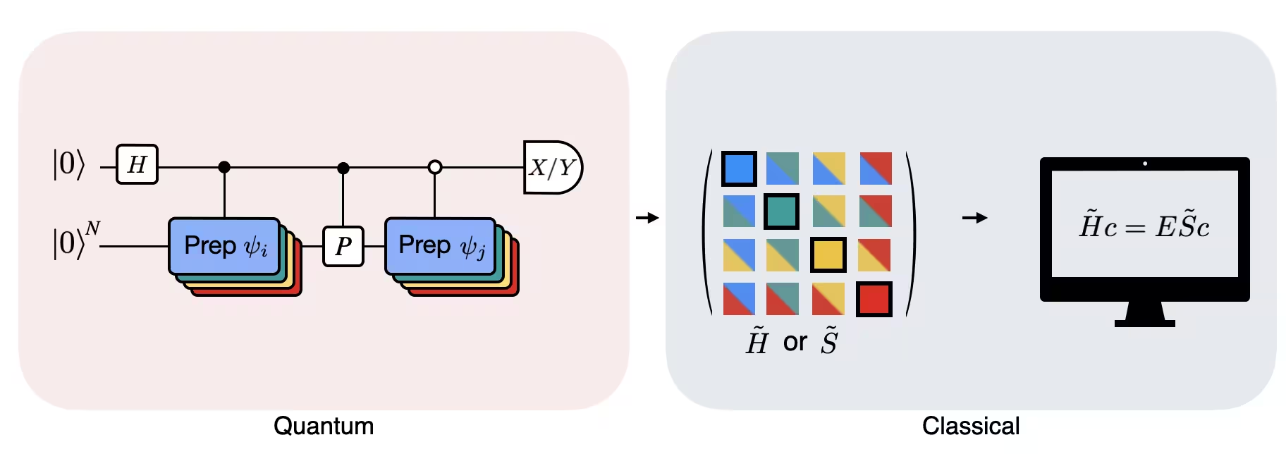
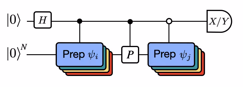
האיור מציג ייצוג מעגל של מבחן הדאמאר המותאם, שיטה המשמשת לחישוב החפיפה בין מצבים קוונטיים שונים. עבור כל אלמנט מטריציאלי $\tilde{H}_{i,j}$, מתבצע מבחן הדאמאר בין המצב $\vert \psi_i \rangle$, $\vert \psi_j \rangle$. זה מודגש באיור על ידי ערכת הצבעים עבור האלמנטים המטריציאליים והפעולות המתאימות $\text{Prep} \; \psi_i$, $\text{Prep} \; \psi_j$. לפיכך, נדרש סט של מבחני הדאמאר עבור כל השילובים האפשריים של וקטורי מרחב קרילוב כדי לחשב את כל האלמנטים המטריציאליים של ההמילטוניאן המוקרן $\tilde{H}$. החוט העליון במעגל מבחן הדאמאר הוא qubit עזר שנמדד בבסיס X או Y, ערך התצפית שלו קובע את הערך של החפיפה בין המצבים. החוט התחתון מייצג את כל ה-qubits של ההמילטוניאן של המערכת. הפעולה $\text{Prep} \; \psi_i$ מכינה את qubit המערכת במצב $\vert \psi_i \rangle$ מותנה במצב של qubit העזר (באופן דומה עבור $\text{Prep} \; \psi_j$) והפעולה $P$ מייצגת פירוק פאולי של ההמילטוניאן של המערכת $H = \sum_i P_i$. גזירה מפורטת יותר של הפעולות המחושבות על ידי מבחן הדאמאר ניתנת להלן.

הגדרת המילטוניאן

בואו נשקול את המילטוניאן הייזנברג עבור $N$ qubits על שרשרת לינארית: $H= \sum_{i,j}^N X_i X_j + Y_i Y_j - J Z_i Z_j$

# Define problem Hamiltonian.
n_qubits = 30
J = 1  # coupling strength for ZZ interaction

# Define the Hamiltonian:
H_int = [["I"] * n_qubits for _ in range(3 * (n_qubits - 1))]
for i in range(n_qubits - 1):
    H_int[i][i] = "Z"
    H_int[i][i + 1] = "Z"
for i in range(n_qubits - 1):
    H_int[n_qubits - 1 + i][i] = "X"
    H_int[n_qubits - 1 + i][i + 1] = "X"
for i in range(n_qubits - 1):
    H_int[2 * (n_qubits - 1) + i][i] = "Y"
    H_int[2 * (n_qubits - 1) + i][i + 1] = "Y"
H_int = ["".join(term) for term in H_int]
H_tot = [(term, J) if term.count("Z") == 2 else (term, 1) for term in H_int]

# Get operator
H_op = SparsePauliOp.from_list(H_tot)
print(H_tot)

[('ZZIIIIIIIIIIIIIIIIIIIIIIIIIIII', 1), ('IZZIIIIIIIIIIIIIIIIIIIIIIIIIII', 1), ('IIZZIIIIIIIIIIIIIIIIIIIIIIIIII', 1), ('IIIZZIIIIIIIIIIIIIIIIIIIIIIIII', 1), ('IIIIZZIIIIIIIIIIIIIIIIIIIIIIII', 1), ('IIIIIZZIIIIIIIIIIIIIIIIIIIIIII', 1), ('IIIIIIZZIIIIIIIIIIIIIIIIIIIIII', 1), ('IIIIIIIZZIIIIIIIIIIIIIIIIIIIII', 1), ('IIIIIIIIZZIIIIIIIIIIIIIIIIIIII', 1), ('IIIIIIIIIZZIIIIIIIIIIIIIIIIIII', 1), ('IIIIIIIIIIZZIIIIIIIIIIIIIIIIII', 1), ('IIIIIIIIIIIZZIIIIIIIIIIIIIIIII', 1), ('IIIIIIIIIIIIZZIIIIIIIIIIIIIIII', 1), ('IIIIIIIIIIIIIZZIIIIIIIIIIIIIII', 1), ('IIIIIIIIIIIIIIZZIIIIIIIIIIIIII', 1), ('IIIIIIIIIIIIIIIZZIIIIIIIIIIIII', 1), ('IIIIIIIIIIIIIIIIZZIIIIIIIIIIII', 1), ('IIIIIIIIIIIIIIIIIZZIIIIIIIIIII', 1), ('IIIIIIIIIIIIIIIIIIZZIIIIIIIIII', 1), ('IIIIIIIIIIIIIIIIIIIZZIIIIIIIII', 1), ('IIIIIIIIIIIIIIIIIIIIZZIIIIIIII', 1), ('IIIIIIIIIIIIIIIIIIIIIZZIIIIIII', 1), ('IIIIIIIIIIIIIIIIIIIIIIZZIIIIII', 1), ('IIIIIIIIIIIIIIIIIIIIIIIZZIIIII', 1), ('IIIIIIIIIIIIIIIIIIIIIIIIZZIIII', 1), ('IIIIIIIIIIIIIIIIIIIIIIIIIZZIII', 1), ('IIIIIIIIIIIIIIIIIIIIIIIIIIZZII', 1), ('IIIIIIIIIIIIIIIIIIIIIIIIIIIZZI', 1), ('IIIIIIIIIIIIIIIIIIIIIIIIIIIIZZ', 1), ('XXIIIIIIIIIIIIIIIIIIIIIIIIIIII', 1), ('IXXIIIIIIIIIIIIIIIIIIIIIIIIIII', 1), ('IIXXIIIIIIIIIIIIIIIIIIIIIIIIII', 1), ('IIIXXIIIIIIIIIIIIIIIIIIIIIIIII', 1), ('IIIIXXIIIIIIIIIIIIIIIIIIIIIIII', 1), ('IIIIIXXIIIIIIIIIIIIIIIIIIIIIII', 1), ('IIIIIIXXIIIIIIIIIIIIIIIIIIIIII', 1), ('IIIIIIIXXIIIIIIIIIIIIIIIIIIIII', 1), ('IIIIIIIIXXIIIIIIIIIIIIIIIIIIII', 1), ('IIIIIIIIIXXIIIIIIIIIIIIIIIIIII', 1), ('IIIIIIIIIIXXIIIIIIIIIIIIIIIIII', 1), ('IIIIIIIIIIIXXIIIIIIIIIIIIIIIII', 1), ('IIIIIIIIIIIIXXIIIIIIIIIIIIIIII', 1), ('IIIIIIIIIIIIIXXIIIIIIIIIIIIIII', 1), ('IIIIIIIIIIIIIIXXIIIIIIIIIIIIII', 1), ('IIIIIIIIIIIIIIIXXIIIIIIIIIIIII', 1), ('IIIIIIIIIIIIIIIIXXIIIIIIIIIIII', 1), ('IIIIIIIIIIIIIIIIIXXIIIIIIIIIII', 1), ('IIIIIIIIIIIIIIIIIIXXIIIIIIIIII', 1), ('IIIIIIIIIIIIIIIIIIIXXIIIIIIIII', 1), ('IIIIIIIIIIIIIIIIIIIIXXIIIIIIII', 1), ('IIIIIIIIIIIIIIIIIIIIIXXIIIIIII', 1), ('IIIIIIIIIIIIIIIIIIIIIIXXIIIIII', 1), ('IIIIIIIIIIIIIIIIIIIIIIIXXIIIII', 1), ('IIIIIIIIIIIIIIIIIIIIIIIIXXIIII', 1), ('IIIIIIIIIIIIIIIIIIIIIIIIIXXIII', 1), ('IIIIIIIIIIIIIIIIIIIIIIIIIIXXII', 1), ('IIIIIIIIIIIIIIIIIIIIIIIIIIIXXI', 1), ('IIIIIIIIIIIIIIIIIIIIIIIIIIIIXX', 1), ('YYIIIIIIIIIIIIIIIIIIIIIIIIIIII', 1), ('IYYIIIIIIIIIIIIIIIIIIIIIIIIIII', 1), ('IIYYIIIIIIIIIIIIIIIIIIIIIIIIII', 1), ('IIIYYIIIIIIIIIIIIIIIIIIIIIIIII', 1), ('IIIIYYIIIIIIIIIIIIIIIIIIIIIIII', 1), ('IIIIIYYIIIIIIIIIIIIIIIIIIIIIII', 1), ('IIIIIIYYIIIIIIIIIIIIIIIIIIIIII', 1), ('IIIIIIIYYIIIIIIIIIIIIIIIIIIIII', 1), ('IIIIIIIIYYIIIIIIIIIIIIIIIIIIII', 1), ('IIIIIIIIIYYIIIIIIIIIIIIIIIIIII', 1), ('IIIIIIIIIIYYIIIIIIIIIIIIIIIIII', 1), ('IIIIIIIIIIIYYIIIIIIIIIIIIIIIII', 1), ('IIIIIIIIIIIIYYIIIIIIIIIIIIIIII', 1), ('IIIIIIIIIIIIIYYIIIIIIIIIIIIIII', 1), ('IIIIIIIIIIIIIIYYIIIIIIIIIIIIII', 1), ('IIIIIIIIIIIIIIIYYIIIIIIIIIIIII', 1), ('IIIIIIIIIIIIIIIIYYIIIIIIIIIIII', 1), ('IIIIIIIIIIIIIIIIIYYIIIIIIIIIII', 1), ('IIIIIIIIIIIIIIIIIIYYIIIIIIIIII', 1), ('IIIIIIIIIIIIIIIIIIIYYIIIIIIIII', 1), ('IIIIIIIIIIIIIIIIIIIIYYIIIIIIII', 1), ('IIIIIIIIIIIIIIIIIIIIIYYIIIIIII', 1), ('IIIIIIIIIIIIIIIIIIIIIIYYIIIIII', 1), ('IIIIIIIIIIIIIIIIIIIIIIIYYIIIII', 1), ('IIIIIIIIIIIIIIIIIIIIIIIIYYIIII', 1), ('IIIIIIIIIIIIIIIIIIIIIIIIIYYIII', 1), ('IIIIIIIIIIIIIIIIIIIIIIIIIIYYII', 1), ('IIIIIIIIIIIIIIIIIIIIIIIIIIIYYI', 1), ('IIIIIIIIIIIIIIIIIIIIIIIIIIIIYY', 1)]

הגדרת פרמטרים לאלגוריתם

אנחנו בוחרים בצורה היוריסטית ערך עבור צעד הזמן dt (בהתבסס על גבולות עליונים על הנורמה של ההמילטוניאן). הפניה [2] הראתה שצעד זמן קטן מספיק הוא $\pi/\vert \vert H \vert \vert$, ושעדיף עד נקודה מסוימת להעריך נמוך את הערך הזה מאשר להעריך גבוה, מכיוון שהערכת יתר יכולה לאפשר תרומות ממצבי אנרגיה גבוהה להשחית אפילו את המצב האופטימלי במרחב קרילוב. מצד שני, בחירת $dt$ קטן מדי מובילה להתניה גרועה יותר של תת-מרחב קרילוב, מכיוון שוקטורי הבסיס קרילוב שונים פחות מצעד זמן לצעד זמן.

# Get Hamiltonian restricted to single-particle states
single_particle_H = np.zeros((n_qubits, n_qubits))
for i in range(n_qubits):
    for j in range(i + 1):
        for p, coeff in H_op.to_list():
            p_x = Pauli(p).x
            p_z = Pauli(p).z
            if all(
                p_x[k] == ((i == k) + (j == k)) % 2 for k in range(n_qubits)
            ):
                sgn = (
                    (-1j) ** sum(p_z[k] and p_x[k] for k in range(n_qubits))
                ) * ((-1) ** p_z[i])
            else:
                sgn = 0
            single_particle_H[i, j] += sgn * coeff
for i in range(n_qubits):
    for j in range(i + 1, n_qubits):
        single_particle_H[i, j] = np.conj(single_particle_H[j, i])

# Set dt according to spectral norm
dt = np.pi / np.linalg.norm(single_particle_H, ord=2)
dt

np.float64(0.10833078115826875)

והגדר פרמטרים אחרים של האלגוריתם. לצורך מדריך זה, נגביל את עצמנו לשימוש במרחב קרילוב עם חמישה ממדים בלבד, שהוא די מגביל.

# Set parameters for quantum Krylov algorithm
krylov_dim = 5  # size of Krylov subspace
num_trotter_steps = 6
dt_circ = dt / num_trotter_steps

הכנת מצב

בחר מצב ייחוס $\vert \psi \rangle$ שיש לו חפיפה מסוימת עם מצב היסוד. עבור המילטוניאן זה, אנחנו משתמשים במצב עם עירור ב-qubit האמצעי $\vert 00..010...00 \rangle$ כמצב הייחוס שלנו.

qc_state_prep = QuantumCircuit(n_qubits)
qc_state_prep.x(int(n_qubits / 2) + 1)
qc_state_prep.draw("mpl", scale=0.5)

אבולוציית זמן

אנחנו יכולים לממש את אופרטור האבולוציה בזמן שנוצר על ידי המילטוניאן נתון: $U=e^{-iHt}$ באמצעות קירוב Lie-Trotter.

t = Parameter("t")

## Create the time-evo op circuit
evol_gate = PauliEvolutionGate(
    H_op, time=t, synthesis=LieTrotter(reps=num_trotter_steps)
)

qr = QuantumRegister(n_qubits)
qc_evol = QuantumCircuit(qr)
qc_evol.append(evol_gate, qargs=qr)

<qiskit.circuit.instructionset.InstructionSet at 0x11eef9be0>

מבחן הדאמאר

$$\begin{equation*} |0\rangle|0\rangle^N \quad\longrightarrow\quad \frac{1}{\sqrt{2}}\Big(|0\rangle + |1\rangle \Big)|0\rangle^N \quad\longrightarrow\quad \frac{1}{\sqrt{2}}\Big(|0\rangle|0\rangle^N+|1\rangle |\psi_i\rangle\Big) \quad\longrightarrow\quad \frac{1}{\sqrt{2}}\Big(|0\rangle |0\rangle^N+|1\rangle P |\psi_i\rangle\Big) \quad\longrightarrow\quad\frac{1}{\sqrt{2}}\Big(|0\rangle |\psi_j\rangle+|1\rangle P|\psi_i\rangle\Big) \end{equation*}$$

כאשר $P$ הוא אחד האיברים בפירוק של ההמילטוניאן $H=\sum P$ ו-$\text{Prep} \; \psi_i$, $\text{Prep} \; \psi_j$ הן פעולות מותנות המכינות $|\psi_i\rangle$, $|\psi_j\rangle$ וקטורים של מרחב קרילוב היוניטרי, עם $|\psi_k\rangle = e^{-i H k dt } \vert \psi \rangle = e^{-i H k dt } U_{\psi} \vert 0 \rangle^N$. כדי למדוד $X$, תחילה יש להחיל $H$...

$$\begin{equation*} \longrightarrow\quad\frac{1}{2}|0\rangle\Big( |\psi_j\rangle + P|\psi_i\rangle\Big) + \frac{1}{2}|1\rangle\Big(|\psi_j\rangle - P|\psi_i\rangle\Big) \end{equation*}$$

... ואז למדוד:

$$\begin{equation*} \begin{split} \Rightarrow\quad\langle X\rangle &= \frac{1}{4}\Bigg(\Big\|| \psi_j\rangle + P|\psi_i\rangle \Big\|^2-\Big\||\psi_j\rangle - P|\psi_i\rangle\Big\|^2\Bigg) \\ &= \text{Re}\Big[\langle\psi_j| P|\psi_i\rangle\Big]. \end{split} \end{equation*}$$

מהזהות $|a + b\|^2 = \langle a + b | a + b \rangle = \|a\|^2 + \|b\|^2 + 2\text{Re}\langle a | b \rangle$. באופן דומה, מדידת $Y$ נותנת

$$\begin{equation*} \langle Y\rangle = \text{Im}\Big[\langle\psi_j| P|\psi_i\rangle\Big]. \end{equation*}$$

## Create the time-evo op circuit
evol_gate = PauliEvolutionGate(
    H_op, time=dt, synthesis=LieTrotter(reps=num_trotter_steps)
)

## Create the time-evo op dagger circuit
evol_gate_d = PauliEvolutionGate(
    H_op, time=dt, synthesis=LieTrotter(reps=num_trotter_steps)
)
evol_gate_d = evol_gate_d.inverse()

# Put pieces together
qc_reg = QuantumRegister(n_qubits)
qc_temp = QuantumCircuit(qc_reg)
qc_temp.compose(qc_state_prep, inplace=True)
for _ in range(num_trotter_steps):
    qc_temp.append(evol_gate, qargs=qc_reg)
for _ in range(num_trotter_steps):
    qc_temp.append(evol_gate_d, qargs=qc_reg)
qc_temp.compose(qc_state_prep.inverse(), inplace=True)

# Create controlled version of the circuit
controlled_U = qc_temp.to_gate().control(1)

# Create hadamard test circuit for real part
qr = QuantumRegister(n_qubits + 1)
qc_real = QuantumCircuit(qr)
qc_real.h(0)
qc_real.append(controlled_U, list(range(n_qubits + 1)))
qc_real.h(0)

print(
    "Circuit for calculating the real part of the overlap in S via Hadamard test"
)
qc_real.draw("mpl", fold=-1, scale=0.5)

Circuit for calculating the real part of the overlap in S via Hadamard test

מעגל מבחן הדאמאר יכול להיות מעגל עמוק ברגע שאנו מפרקים לשערים מקוריים (שיגדל עוד יותר אם ניקח בחשבון את הטופולוגיה של המכשיר)

print(
    "Number of layers of 2Q operations",
    qc_real.decompose(reps=2).depth(lambda x: x[0].num_qubits == 2),
)

Number of layers of 2Q operations 112753

שלב 2: אופטימיזציה של הבעיה לביצוע על חומרה קוונטית

מבחן הדאמאר יעיל

אנחנו יכולים לבצע אופטימיזציה של המעגלים העמוקים עבור מבחן הדאמאר שקיבלנו על ידי הכנסת קירובים מסוימים והסתמכות על כמה הנחות לגבי המילטוניאן המודל. לדוגמה, שקול את המעגל הבא עבור מבחן הדאמאר:

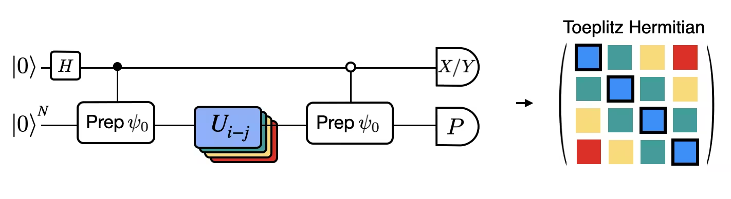
נניח שאנחנו יכולים לחשב באופן קלאסי את $E_0$, הערך העצמי של $|0\rangle^N$ תחת ההמילטוניאן $H$. זה מתקיים כאשר ההמילטוניאן משמר את הסימטריה U(1). למרות שזה עשוי להיראות כהנחה חזקה, ישנם מקרים רבים שבהם בטוח להניח שיש מצב ואקום (במקרה זה הוא ממפה למצב $|0\rangle^N$) שלא מושפע מפעולת ההמילטוניאן. זה נכון למשל עבור המילטוניאנים כימיים המתארים מולקולה יציבה (כאשר מספר האלקטרונים נשמר). בהינתן שהשער $\text{Prep} \; \psi$, מכין את מצב הייחוס הרצוי $\ket{psi} = \text{Prep} \; \psi \ket{0} = e^{-i H 0 dt} U_{\psi} \ket{0}$, לדוגמה, כדי להכין את מצב ה-HF עבור כימיה $\text{Prep} \; \psi$ יהיה מכפלה של NOTs של qubit יחיד, לכן controlled-$\text{Prep} \; \psi$ הוא רק מכפלה של CNOTs. לאחר מכן המעגל לעיל מיישם את המצב הבא לפני המדידה:

$$\begin{equation} \begin{split} \ket{0} \ket{0}^N\xrightarrow{H}&\frac{1}{\sqrt{2}} \left( \ket{0}\ket{0}^N+ \ket{1} \ket{0}^N \right)\\ \xrightarrow{\text{1-ctrl-init}}&\frac{1}{\sqrt{2}}\left(|0\rangle|0\rangle^N+|1\rangle|\psi\rangle\right)\\ \xrightarrow{U}&\frac{1}{\sqrt{2}}\left(e^{i\phi}\ket{0}\ket{0}^N+\ket{1} U\ket{\psi}\right)\\ \xrightarrow{\text{0-ctrl-init}}&\frac{1}{\sqrt{2}} \left( e^{i\phi}\ket{0} \ket{\psi} +\ket{1} U\ket{\psi} \right)\\ =&\frac{1}{2} \left( \ket{+}\left(e^{i\phi}\ket{\psi}+U\ket{\psi}\right) +\ket{-}\left(e^{i\phi}\ket{\psi}-U\ket{\psi}\right) \right)\\ =&\frac{1}{2} \left( \ket{+i}\left(e^{i\phi}\ket{\psi}-iU\ket{\psi}\right) +\ket{-i}\left(e^{i\phi}\ket{\psi}+iU\ket{\psi}\right) \right) \end{split} \end{equation}$$

כאשר השתמשנו בהסטת פאזה הניתנת לסימולציה קלאסית $U\ket{0}^N = e^{i\phi}\ket{0}^N$ בשורה השלישית. לכן ערכי התצפית מתקבלים כ

$$\begin{equation} \begin{split} \langle X\otimes P\rangle&=\frac{1}{4} \Big( \left(e^{-i\phi}\bra{\psi}+\bra{\psi}U^\dagger\right)P\left(e^{i\phi}\ket{\psi}+U\ket{\psi}\right) \\ &\qquad-\left(e^{-i\phi}\bra{\psi}-\bra{\psi}U^\dagger\right)P\left(e^{i\phi}\ket{\psi}-U\ket{\psi}\right) \Big)\\ &=\text{Re}\left[e^{-i\phi}\bra{\psi}PU\ket{\psi}\right], \end{split} \end{equation}$$ $$\begin{equation} \begin{split} \langle Y\otimes P\rangle&=\frac{1}{4} \Big( \left(e^{-i\phi}\bra{\psi}+i\bra{\psi}U^\dagger\right)P\left(e^{i\phi}\ket{\psi}-iU\ket{\psi}\right) \\ &\qquad-\left(e^{-i\phi}\bra{\psi}-i\bra{\psi}U^\dagger\right)P\left(e^{i\phi}\ket{\psi}+iU\ket{\psi}\right) \Big)\\ &=\text{Im}\left[e^{-i\phi}\bra{\psi}PU\ket{\psi}\right]. \end{split} \end{equation}$$

באמצעות הנחות אלה היינו מסוגלים לכתוב את ערכי התצפית של אופרטורים בעלי עניין עם פחות פעולות מותנות. למעשה, אנחנו צריכים רק ליישם את הכנת המצב המותנית $\text{Prep} \; \psi$ ולא אבולוציות זמן מותנות. ניסוח מחדש של החישוב שלנו כאמור לעיל יאפשר לנו להפחית מאוד את העומק של המעגלים המתקבלים.

פירוק אופרטור אבולוציית הזמן עם פירוק טרוטר

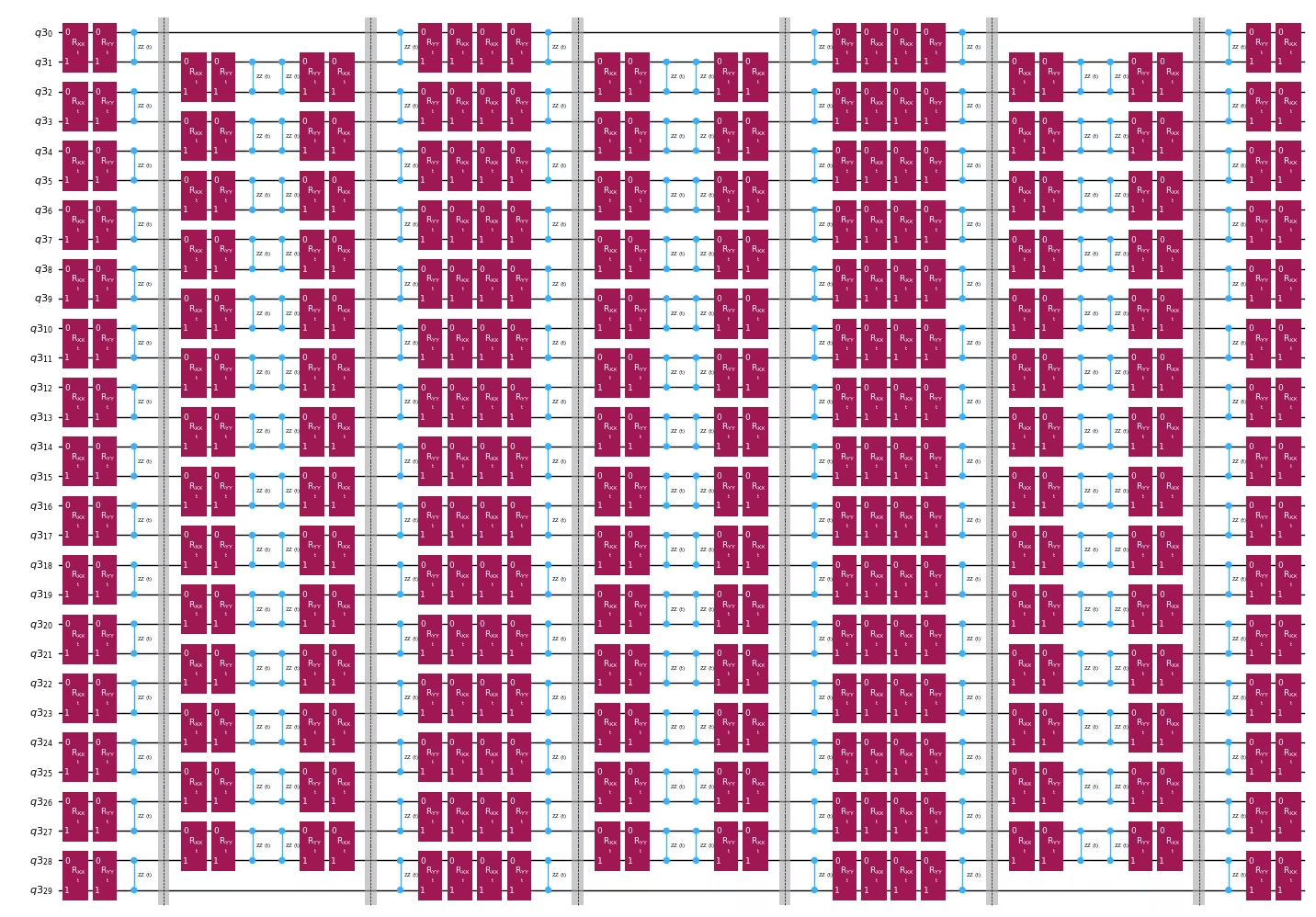
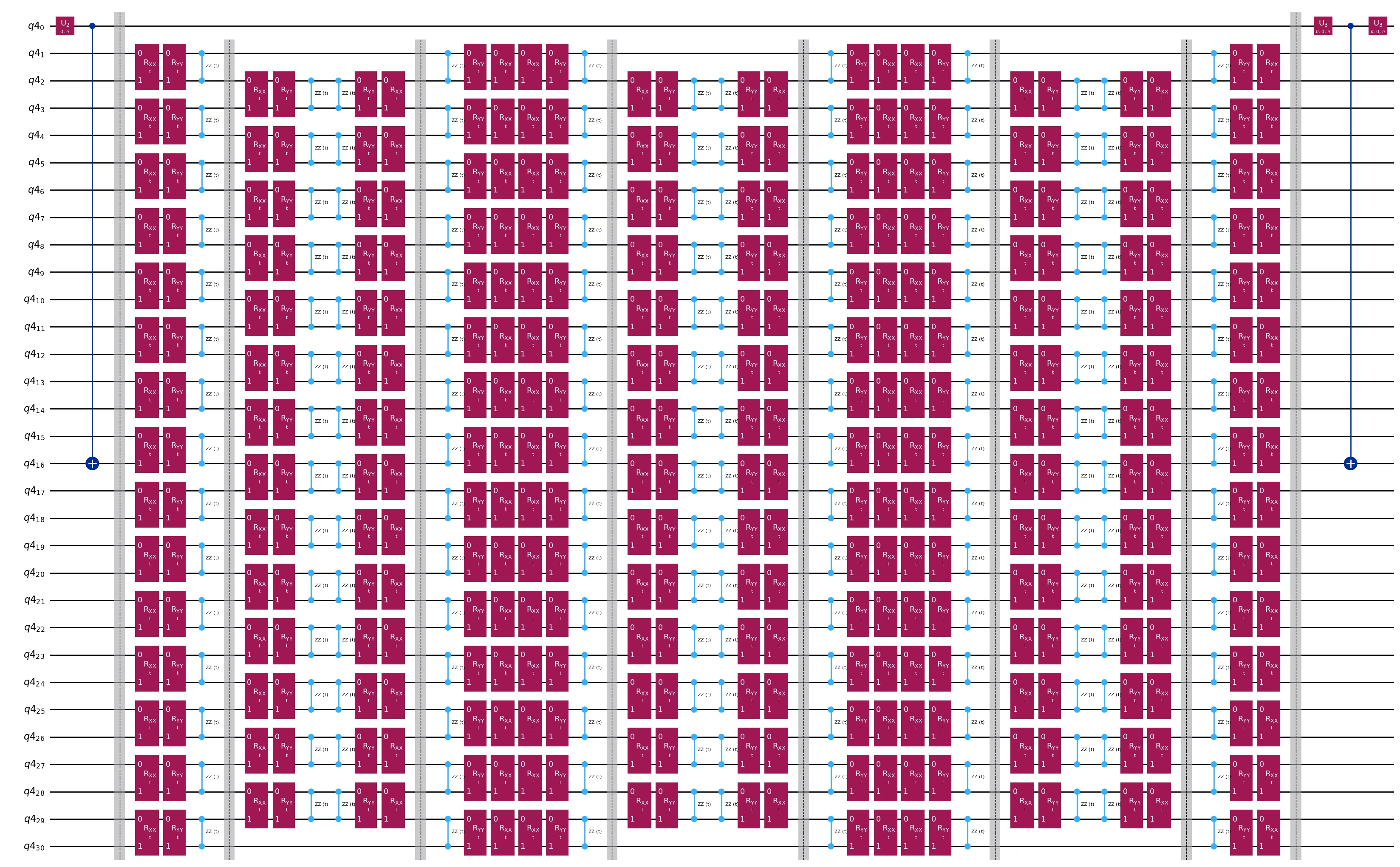
במקום ליישם את אופרטור אבולוציית הזמן בדיוק אנחנו יכולים להשתמש בפירוק טרוטר כדי ליישם קירוב שלו. חזרה מספר פעמים על פירוק טרוטר של סדר מסוים נותנת לנו הפחתה נוספת של השגיאה שהוכנסה מהקירוב. בהמשך, אנחנו בונים ישירות את יישום טרוטר בצורה היעילה ביותר עבור גרף האינטראקציה של ההמילטוניאן שאנו שוקלים (אינטראקציות שכנים קרובים בלבד). בפועל אנחנו מכניסים סיבובי פאולי $R_{xx}$, $R_{yy}$, $R_{zz}$ עם זווית מפרמטרית $t$ התואמים ליישום המקורב של $e^{-i (XX + YY + ZZ) t}$. בהינתן ההבדל בהגדרה של סיבובי פאולי ואבולוציית הזמן שאנו מנסים ליישם, נצטרך להשתמש בפרמטר $2*dt$ כדי להשיג אבולוציית זמן של $dt$. יתר על כן, אנחנו הופכים את סדר הפעולות עבור מספר אי-זוגי של חזרות של שלבי טרוטר, שהוא שווה ערך פונקציונלי אך מאפשר סינתזה של פעולות סמוכות ביוניטרי $SU(2)$ יחיד. זה נותן מעגל הרבה יותר רדוד ממה שמתקבל באמצעות הפונקציונליות הגנרית PauliEvolutionGate().

t = Parameter("t")

# Create instruction for rotation about XX+YY-ZZ:
Rxyz_circ = QuantumCircuit(2)
Rxyz_circ.rxx(t, 0, 1)
Rxyz_circ.ryy(t, 0, 1)
Rxyz_circ.rzz(t, 0, 1)
Rxyz_instr = Rxyz_circ.to_instruction(label="RXX+YY+ZZ")

interaction_list = [
    [[i, i + 1] for i in range(0, n_qubits - 1, 2)],
    [[i, i + 1] for i in range(1, n_qubits - 1, 2)],
]  # linear chain

qr = QuantumRegister(n_qubits)
trotter_step_circ = QuantumCircuit(qr)
for i, color in enumerate(interaction_list):
    for interaction in color:
        trotter_step_circ.append(Rxyz_instr, interaction)
    if i < len(interaction_list) - 1:
        trotter_step_circ.barrier()
reverse_trotter_step_circ = trotter_step_circ.reverse_ops()

qc_evol = QuantumCircuit(qr)
for step in range(num_trotter_steps):
    if step % 2 == 0:
        qc_evol = qc_evol.compose(trotter_step_circ)
    else:
        qc_evol = qc_evol.compose(reverse_trotter_step_circ)

qc_evol.decompose().draw("mpl", fold=-1, scale=0.5)

שימוש במעגל מותאם להכנת מצב

control = 0
excitation = int(n_qubits / 2) + 1
controlled_state_prep = QuantumCircuit(n_qubits + 1)
controlled_state_prep.cx(control, excitation)
controlled_state_prep.draw("mpl", fold=-1, scale=0.5)

תבניות מעגלים לחישוב אלמנטים מטריציאליים של $\tilde{S}$ ו-$\tilde{H}$ באמצעות מבחן הדאמאר

ההבדל היחיד בין המעגלים המשמשים במבחן הדאמאר יהיה הפאזה באופרטור אבולוציית הזמן והתצפיות הנמדדות. לכן אנחנו יכולים להכין תבנית מעגל המייצגת את המעגל הגנרי עבור מבחן הדאמאר, עם מצייני מיקום עבור השערים שתלויים באופרטור אבולוציית הזמן.

# Parameters for the template circuits
parameters = []
for idx in range(1, krylov_dim):
    parameters.append(2 * dt_circ * (idx))

# Create modified hadamard test circuit
qr = QuantumRegister(n_qubits + 1)
qc = QuantumCircuit(qr)
qc.h(0)
qc.compose(controlled_state_prep, list(range(n_qubits + 1)), inplace=True)
qc.barrier()
qc.compose(qc_evol, list(range(1, n_qubits + 1)), inplace=True)
qc.barrier()
qc.x(0)
qc.compose(
    controlled_state_prep.inverse(), list(range(n_qubits + 1)), inplace=True
)
qc.x(0)

qc.decompose().draw("mpl", fold=-1)

print(
    "The optimized circuit has 2Q gates depth: ",
    qc.decompose().decompose().depth(lambda x: x[0].num_qubits == 2),
)

The optimized circuit has 2Q gates depth:  74

הפחתנו באופן ניכר את העומק של מבחן הדאמאר עם שילוב של קירוב טרוטר ויוניטריים לא-מותנים

שלב 3: ביצוע באמצעות פרימיטיבים של Qiskit

יצירת מופע של ה-backend והגדרת פרמטרי זמן ריצה

service = QiskitRuntimeService()
backend = service.least_busy(operational=True, simulator=False)
if (
    "if_else" not in backend.target.operation_names
):  # Needed as "op_name" could be "if_else"
    backend.target.add_instruction(IfElseOp, name="if_else")
print(backend.name)

Transpiling ל-QPU

ראשית, בואו נבחר תת-קבוצות של מפת הצימוד עם qubits בעלי ביצועים "טובים" (כאשר "טוב" הוא די שרירותי כאן, אנחנו בעיקר רוצים להימנע מ-qubits בעלי ביצועים ממש גרועים) וליצור target חדש עבור transpilation

target = backend.target
cmap = target.build_coupling_map(filter_idle_qubits=True)
cmap_list = list(cmap.get_edges())

cust_cmap_list = copy.deepcopy(cmap_list)
for q in range(target.num_qubits):
    meas_err = target["measure"][(q,)].error
    t2 = target.qubit_properties[q].t2 * 1e6
    if meas_err > 0.02 or t2 < 100:
        for q_pair in cmap_list:
            if q in q_pair:
                try:
                    cust_cmap_list.remove(q_pair)
                except:
                    continue

for q in cmap_list:
    op_name = list(target.operation_names_for_qargs(q))[0]
    twoq_gate_err = target[f"{op_name}"][q].error
    if twoq_gate_err > 0.005:
        for q_pair in cmap_list:
            if q == q_pair:
                try:
                    cust_cmap_list.remove(q)
                except:
                    continue

cust_cmap = CouplingMap(cust_cmap_list)
cust_target = Target.from_configuration(
    basis_gates=backend.configuration().basis_gates,
    coupling_map=cust_cmap,
)

לאחר מכן בצע transpile של המעגל הוירטואלי לפריסה הפיזית הטובה ביותר ב-target החדש הזה

basis_gates = list(target.operation_names)
pm = generate_preset_pass_manager(
    optimization_level=3,
    target=cust_target,
    basis_gates=basis_gates,
)

qc_trans = pm.run(qc)

print("depth", qc_trans.depth(lambda x: x[0].num_qubits == 2))
print("num 2q ops", qc_trans.count_ops())
print(
    "physical qubits",
    sorted(
        [
            idx
            for idx, qb in qc_trans.layout.initial_layout.get_physical_bits().items()
            if qb._register.name != "ancilla"
        ]
    ),
)

depth 52
num 2q ops OrderedDict([('rz', 2058), ('sx', 1703), ('cz', 728), ('x', 84), ('barrier', 8)])
physical qubits [91, 92, 93, 94, 95, 98, 99, 108, 109, 110, 111, 113, 114, 115, 119, 127, 132, 133, 134, 135, 137, 139, 147, 148, 149, 150, 151, 152, 153, 154, 155]

יצירת PUBs לביצוע עם Estimator

# Define observables to measure for S
observable_S_real = "I" * (n_qubits) + "X"
observable_S_imag = "I" * (n_qubits) + "Y"

observable_op_real = SparsePauliOp(
    observable_S_real
)  # define a sparse pauli operator for the observable
observable_op_imag = SparsePauliOp(observable_S_imag)

layout = qc_trans.layout  # get layout of transpiled circuit
observable_op_real = observable_op_real.apply_layout(
    layout
)  # apply physical layout to the observable
observable_op_imag = observable_op_imag.apply_layout(layout)
observable_S_real = (
    observable_op_real.paulis.to_labels()
)  # get the label of the physical observable
observable_S_imag = observable_op_imag.paulis.to_labels()

observables_S = [[observable_S_real], [observable_S_imag]]

# Define observables to measure for H
# Hamiltonian terms to measure
observable_list = []
for pauli, coeff in zip(H_op.paulis, H_op.coeffs):
    # print(pauli)
    observable_H_real = pauli[::-1].to_label() + "X"
    observable_H_imag = pauli[::-1].to_label() + "Y"
    observable_list.append([observable_H_real])
    observable_list.append([observable_H_imag])

layout = qc_trans.layout

observable_trans_list = []
for observable in observable_list:
    observable_op = SparsePauliOp(observable)
    observable_op = observable_op.apply_layout(layout)
    observable_trans_list.append([observable_op.paulis.to_labels()])

observables_H = observable_trans_list

# Define a sweep over parameter values
params = np.vstack(parameters).T

# Estimate the expectation value for all combinations of
# observables and parameter values, where the pub result will have
# shape (# observables, # parameter values).
pub = (qc_trans, observables_S + observables_H, params)

הרצת מעגלים

מעגלים עבור $t=0$ ניתנים לחישוב קלאסי

qc_cliff = qc.assign_parameters({t: 0})

# Get expectation values from experiment
S_expval_real = StabilizerState(qc_cliff).expectation_value(
    Pauli("I" * (n_qubits) + "X")
)
S_expval_imag = StabilizerState(qc_cliff).expectation_value(
    Pauli("I" * (n_qubits) + "Y")
)

# Get expectation values
S_expval = S_expval_real + 1j * S_expval_imag

H_expval = 0
for obs_idx, (pauli, coeff) in enumerate(zip(H_op.paulis, H_op.coeffs)):
    # Get expectation values from experiment
    expval_real = StabilizerState(qc_cliff).expectation_value(
        Pauli(pauli[::-1].to_label() + "X")
    )
    expval_imag = StabilizerState(qc_cliff).expectation_value(
        Pauli(pauli[::-1].to_label() + "Y")
    )
    expval = expval_real + 1j * expval_imag

    # Fill-in matrix elements
    H_expval += coeff * expval

print(H_expval)

(25+0j)

ביצוע מעגלים עבור $S$ ו-$\tilde{H}$ עם ה-Estimator

# Experiment options
num_randomizations = 300
num_randomizations_learning = 30
shots_per_randomization = 100
noise_factors = [1, 1.2, 1.4]
learning_pair_depths = [0, 4, 24, 48]

experimental_opts = {}
experimental_opts["resilience"] = {
    "measure_mitigation": True,
    "measure_noise_learning": {
        "num_randomizations": num_randomizations_learning,
        "shots_per_randomization": shots_per_randomization,
    },
    "zne_mitigation": True,
    "zne": {"noise_factors": noise_factors},
    "layer_noise_learning": {
        "max_layers_to_learn": 10,
        "layer_pair_depths": learning_pair_depths,
        "shots_per_randomization": shots_per_randomization,
        "num_randomizations": num_randomizations_learning,
    },
    "zne": {
        "amplifier": "pea",
        "extrapolated_noise_factors": [0] + noise_factors,
    },
}
experimental_opts["twirling"] = {
    "num_randomizations": num_randomizations,
    "shots_per_randomization": shots_per_randomization,
    "strategy": "all",
}

estimator = Estimator(mode=backend, options=experimental_opts)

job = estimator.run([pub])

שלב 4: עיבוד לאחר והחזרת תוצאה בפורמט קלאסי רצוי

results = job.result()[0]

חישוב מטריצות המילטוניאן אפקטיבי וחפיפה

ראשית חשב את הפאזה שנצברת על ידי המצב $\vert 0 \rangle$ במהלך אבולוציית הזמן הלא-מותנית

prefactors = [
    np.exp(-1j * sum([c for p, c in H_op.to_list() if "Z" in p]) * i * dt)
    for i in range(1, krylov_dim)
]

ברגע שיש לנו את התוצאות של ביצועי המעגל אנחנו יכולים לבצע עיבוד מאוחר של הנתונים כדי לחשב את האלמנטים המטריציאליים של $S$

# Assemble S, the overlap matrix of dimension D:
S_first_row = np.zeros(krylov_dim, dtype=complex)
S_first_row[0] = 1 + 0j

# Add in ancilla-only measurements:
for i in range(krylov_dim - 1):
    # Get expectation values from experiment
    expval_real = results.data.evs[0][0][
        i
    ]  # automatic extrapolated evs if ZNE is used
    expval_imag = results.data.evs[1][0][
        i
    ]  # automatic extrapolated evs if ZNE is used

    # Get expectation values
    expval = expval_real + 1j * expval_imag
    S_first_row[i + 1] += prefactors[i] * expval

S_first_row_list = S_first_row.tolist()  # for saving purposes

S_circ = np.zeros((krylov_dim, krylov_dim), dtype=complex)

# Distribute entries from first row across matrix:
for i, j in it.product(range(krylov_dim), repeat=2):
    if i >= j:
        S_circ[j, i] = S_first_row[i - j]
    else:
        S_circ[j, i] = np.conj(S_first_row[j - i])

Matrix(S_circ)

$$\displaystyle \left[\begin{matrix}1.0 & -0.723052998582984 - 0.345085413575966 i & 0.467051960502366 + 0.516197865254034 i & -0.180546747798251 - 0.492624093654174 i & 0.0012070853532697 + 0.312052218182462 i\\-0.723052998582984 + 0.345085413575966 i & 1.0 & -0.723052998582984 - 0.345085413575966 i & 0.467051960502366 + 0.516197865254034 i & -0.180546747798251 - 0.492624093654174 i\\0.467051960502366 - 0.516197865254034 i & -0.723052998582984 + 0.345085413575966 i & 1.0 & -0.723052998582984 - 0.345085413575966 i & 0.467051960502366 + 0.516197865254034 i\\-0.180546747798251 + 0.492624093654174 i & 0.467051960502366 - 0.516197865254034 i & -0.723052998582984 + 0.345085413575966 i & 1.0 & -0.723052998582984 - 0.345085413575966 i\\0.0012070853532697 - 0.312052218182462 i & -0.180546747798251 + 0.492624093654174 i & 0.467051960502366 - 0.516197865254034 i & -0.723052998582984 + 0.345085413575966 i & 1.0\end{matrix}\right]$$

והאלמנטים המטריציאליים של $\tilde{H}$

# Assemble S, the overlap matrix of dimension D:
H_first_row = np.zeros(krylov_dim, dtype=complex)
H_first_row[0] = H_expval

for obs_idx, (pauli, coeff) in enumerate(zip(H_op.paulis, H_op.coeffs)):
    # Add in ancilla-only measurements:
    for i in range(krylov_dim - 1):
        # Get expectation values from experiment
        expval_real = results.data.evs[2 + 2 * obs_idx][0][
            i
        ]  # automatic extrapolated evs if ZNE is used
        expval_imag = results.data.evs[2 + 2 * obs_idx + 1][0][
            i
        ]  # automatic extrapolated evs if ZNE is used

        # Get expectation values
        expval = expval_real + 1j * expval_imag
        H_first_row[i + 1] += prefactors[i] * coeff * expval

H_first_row_list = H_first_row.tolist()

H_eff_circ = np.zeros((krylov_dim, krylov_dim), dtype=complex)

# Distribute entries from first row across matrix:
for i, j in it.product(range(krylov_dim), repeat=2):
    if i >= j:
        H_eff_circ[j, i] = H_first_row[i - j]
    else:
        H_eff_circ[j, i] = np.conj(H_first_row[j - i])

Matrix(H_eff_circ)

$$\displaystyle \left[\begin{matrix}25.0 & -14.2437089383409 - 6.50486277982165 i & 10.2857217968584 + 9.0431912203186 i & -5.15587257589417 - 8.88280836036843 i & 1.98818301405581 + 5.8897614762563 i\\-14.2437089383409 + 6.50486277982165 i & 25.0 & -14.2437089383409 - 6.50486277982165 i & 10.2857217968584 + 9.0431912203186 i & -5.15587257589417 - 8.88280836036843 i\\10.2857217968584 - 9.0431912203186 i & -14.2437089383409 + 6.50486277982165 i & 25.0 & -14.2437089383409 - 6.50486277982165 i & 10.2857217968584 + 9.0431912203186 i\\-5.15587257589417 + 8.88280836036843 i & 10.2857217968584 - 9.0431912203186 i & -14.2437089383409 + 6.50486277982165 i & 25.0 & -14.2437089383409 - 6.50486277982165 i\\1.98818301405581 - 5.8897614762563 i & -5.15587257589417 + 8.88280836036843 i & 10.2857217968584 - 9.0431912203186 i & -14.2437089383409 + 6.50486277982165 i & 25.0\end{matrix}\right]$$

לבסוף, אנחנו יכולים לפתור את בעיית הערך העצמי המוכללת עבור $\tilde{H}$:

$\tilde{H} \vec{c} = c S \vec{c}$

ולקבל הערכה של אנרגיית מצב היסוד $c_{min}$

gnd_en_circ_est_list = []
for d in range(1, krylov_dim + 1):
    # Solve generalized eigenvalue problem for different size of the Krylov space
    gnd_en_circ_est = solve_regularized_gen_eig(
        H_eff_circ[:d, :d], S_circ[:d, :d], threshold=9e-1
    )
    gnd_en_circ_est_list.append(gnd_en_circ_est)
    print("The estimated ground state energy is: ", gnd_en_circ_est)

The estimated ground state energy is:  25.0
The estimated ground state energy is:  22.572154819954875
The estimated ground state energy is:  21.691509219286587
The estimated ground state energy is:  21.23882298756386
The estimated ground state energy is:  20.965499325470294

עבור סקטור חלקיק יחיד, אנחנו יכולים לחשב ביעילות את מצב היסוד של סקטור זה של ההמילטוניאן באופן קלאסי

gs_en = single_particle_gs(H_op, n_qubits)

n_sys_qubits 30
n_exc 1 , subspace dimension 31
single particle ground state energy:  21.021912418526906

plt.plot(
    range(1, krylov_dim + 1),
    gnd_en_circ_est_list,
    color="blue",
    linestyle="-.",
    label="KQD estimate",
)
plt.plot(
    range(1, krylov_dim + 1),
    [gs_en] * krylov_dim,
    color="red",
    linestyle="-",
    label="exact",
)
plt.xticks(range(1, krylov_dim + 1), range(1, krylov_dim + 1))
plt.legend()
plt.xlabel("Krylov space dimension")
plt.ylabel("Energy")
plt.title(
    "Estimating Ground state energy with Krylov Quantum Diagonalization"
)
plt.show()

נספח: תת-מרחב קרילוב מאבולוציות זמן אמיתיות

מרחב קרילוב היוניטרי מוגדר כ

$$\mathcal{K}_U(H, |\psi\rangle) = \text{span}\left\{ |\psi\rangle, e^{-iH\,dt} |\psi\rangle, \dots, e^{-irH\,dt} |\psi\rangle \right\}$$

עבור צעד זמן $dt$ שנקבע מאוחר יותר. נניח זמנית ש-$r$ זוגי: אז נגדיר $d=r/2$. שים לב שכאשר אנחנו מקרינים את ההמילטוניאן למרחב קרילוב לעיל, הוא בלתי ניתן להבחנה ממרחב קרילוב

$$\mathcal{K}_U(H, |\psi\rangle) = \text{span}\left\{ e^{i\,d\,H\,dt}|\psi\rangle, e^{i(d-1)H\,dt} |\psi\rangle, \dots, e^{-i(d-1)H\,dt} |\psi\rangle, e^{-i\,d\,H\,dt} |\psi\rangle \right\},$$

כלומר, כאשר כל אבולוציות הזמן מוסטות לאחור ב-$d$ צעדי זמן. הסיבה שהוא בלתי ניתן להבחנה היא כי האלמנטים המטריציאליים

$$\tilde{H}_{j,k} = \langle\psi|e^{i\,j\,H\,dt}He^{-i\,k\,H\,dt}|\psi\rangle=\langle\psi|He^{i(j-k)H\,dt}|\psi\rangle$$

אינם משתנים תחת הסטות כלליות של זמן האבולוציה, מכיוון שאבולוציות הזמן מתחלפות עם ההמילטוניאן. עבור $r$ אי-זוגי, אנחנו יכולים להשתמש בניתוח עבור $r-1$.

אנחנו רוצים להראות שאיפשהו במרחב קרילוב הזה, יש ערובה שיהיה מצב אנרגיה נמוכה. אנחנו עושים זאת באמצעות התוצאה הבאה, שנגזרת ממשפט 3.1 ב-[3]:

טענה 1: קיימת פונקציה $f$ כך שעבור אנרגיות $E$ בטווח הספקטרלי של ההמילטוניאן (כלומר, בין אנרגיית מצב היסוד לאנרגיה המקסימלית)...

1. $f(E_0)=1$
2. $|f(E)|\le2\left(1 + \delta\right)^{-d}$ עבור כל הערכים של $E$ שנמצאים $\ge\delta$ הרחק מ-$E_0$, כלומר, היא מדוכאת באופן אקספוננציאלי
3. $f(E)$ היא צירוף לינארי של $e^{ijE\,dt}$ עבור $j=-d,-d+1,...,d-1,d$

אנחנו נותנים הוכחה להלן, אך ניתן לדלג עליה בבטחה אלא אם רוצים להבין את הטיעון המלא והקפדני. לעת עתה אנחנו מתמקדים בהשלכות של הטענה לעיל. לפי תכונה 3 לעיל, אנחנו יכולים לראות שמרחב קרילוב המוסט לעיל מכיל את המצב $f(H)|\psi\rangle$. זהו מצב האנרגיה הנמוכה שלנו. כדי לראות למה, כתוב את $|\psi\rangle$ בבסיס האנרגיה העצמית:

$$|\psi\rangle = \sum_{k=0}^{N}\gamma_k|E_k\rangle,$$

כאשר $|E_k\rangle$ הוא המצב העצמי האנרגטי ה-k ו-$\gamma_k$ היא האמפליטודה שלו במצב ההתחלתי $|\psi\rangle$. מבוטא במונחים של זה, $f(H)|\psi\rangle$ ניתן על ידי

$$f(H)|\psi\rangle = \sum_{k=0}^{N}\gamma_kf(E_k)|E_k\rangle,$$

באמצעות העובדה שאנחנו יכולים להחליף את $H$ ב-$E_k$ כאשר הוא פועל על המצב העצמי $|E_k\rangle$. שגיאת האנרגיה של מצב זה היא לכן

$$\text{energy error} = \frac{\langle\psi|f(H)(H-E_0)f(H)|\psi\rangle}{\langle\psi|f(H)^2|\psi\rangle}$$ $$= \frac{\sum_{k=0}^{N}|\gamma_k|^2f(E_k)^2(E_k-E_0)}{\sum_{k=0}^{N}|\gamma_k|^2f(E_k)^2}.$$

כדי להפוך את זה לגבול עליון שקל יותר להבין, אנחנו קודם כל מפרידים את הסכום במונה לאיברים עם $E_k-E_0\le\delta$ ואיברים עם $E_k-E_0>\delta$:

$$\text{energy error} = \frac{\sum_{E_k\le E_0+\delta}|\gamma_k|^2f(E_k)^2(E_k-E_0)}{\sum_{k=0}^{N}|\gamma_k|^2f(E_k)^2} + \frac{\sum_{E_k> E_0+\delta}|\gamma_k|^2f(E_k)^2(E_k-E_0)}{\sum_{k=0}^{N}|\gamma_k|^2f(E_k)^2}.$$

אנחנו יכולים להגביל את האיבר הראשון מלמעלה על ידי $\delta$,

$$\frac{\sum_{E_k\le E_0+\delta}|\gamma_k|^2f(E_k)^2(E_k-E_0)}{\sum_{k=0}^{N}|\gamma_k|^2f(E_k)^2} < \frac{\delta\sum_{E_k\le E_0+\delta}|\gamma_k|^2f(E_k)^2}{\sum_{k=0}^{N}|\gamma_k|^2f(E_k)^2} \le \delta,$$

כאשר השלב הראשון נובע מכך ש-$E_k-E_0\le\delta$ עבור כל $E_k$ בסכום, והשלב השני נובע מכך שהסכום במונה הוא תת-קבוצה של הסכום במכנה. עבור האיבר השני, ראשית אנחנו מגבילים את המכנה מלמטה על ידי $|\gamma_0|^2$, מכיוון ש-$f(E_0)^2=1$: חיבור הכל בחזרה ביחד, זה נותן

$$\text{energy error} \le \delta + \frac{1}{|\gamma_0|^2}\sum_{E_k>E_0+\delta}|\gamma_k|^2f(E_k)^2(E_k-E_0).$$

כדי לפשט את מה שנשאר, שים לב שעבור כל ה-$E_k$ האלה, לפי ההגדרה של $f$ אנחנו יודעים ש-$f(E_k)^2 \le 4\left(1 + \delta\right)^{-2d}$. בנוסף הגבלה מלמעלה של $E_k-E_0<2\|H\|$ והגבלה מלמעלה של $\sum_{E_k>E_0+\delta}|\gamma_k|^2<1$ נותנת

$$\text{energy error} \le \delta + \frac{8}{|\gamma_0|^2}\|H\|\left(1 + \delta\right)^{-2d}.$$

זה מתקיים עבור כל $\delta>0$, לכן אם נגדיר את $\delta$ שווה לשגיאת המטרה שלנו, אז גבול השגיאה לעיל מתכנס לכך באופן אקספוננציאלי עם ממד קרילוב $2d=r$. שים לב גם שאם $\delta<E_1-E_0$ אז איבר ה-$\delta$ בעצם נעלם לחלוטין בגבול לעיל.

כדי להשלים את הטיעון, ראשית נציין שהנ"ל הוא רק שגיאת האנרגיה של המצב המסוים $f(H)|\psi\rangle$, ולא שגיאת האנרגיה של מצב האנרגיה הנמוכה ביותר במרחב קרילוב. עם זאת, על פי עקרון (Rayleigh-Ritz) וריאציוני, שגיאת האנרגיה של מצב האנרגיה הנמוכה ביותר במרחב קרילוב מוגבלת מלמעלה על ידי שגיאת האנרגיה של כל מצב במרחב קרילוב, כך שהנ"ל הוא גם גבול עליון על שגיאת האנרגיה של מצב האנרגיה הנמוכה ביותר, כלומר, הפלט של אלגוריתם האלכסון הקוונטי קרילוב.

ניתוח דומה כמו לעיל ניתן לבצע שגם מתחשב ברעש ובהליך הסף שנדון במחברת. ראה [2] ו-[4] עבור ניתוח זה.

נספח: הוכחה של טענה 1

הדברים הבאים נגזרים בעיקר מ-[3], משפט 3.1: תן $0 < a < b$ ותן $\Pi^*_d$ להיות מרחב הפולינומים השייריים (פולינומים שערכם ב-0 הוא 1) מדרגה לכל היותר $d$. הפתרון ל

$$\beta(a, b, d) = \min_{p \in \Pi^*_d} \max_{x \in [a, b]} |p(x)| \quad$$

הוא

$$p^*(x) = \frac{T_d\left(\frac{b + a - 2x}{b - a}\right)}{T_d\left(\frac{b + a}{b - a}\right)}, \quad$$

והערך המינימלי המתאים הוא

$$\beta(a, b, d) = T_d^{-1}\left(\frac{b + a}{b - a}\right).$$

אנחנו רוצים להמיר את זה לפונקציה שניתן לבטא באופן טבעי במונחים של אקספוננציאלים מרוכבים, כי אלו הן אבולוציות הזמן האמיתיות שיוצרות את מרחב קרילוב הקוונטי. כדי לעשות זאת, נוח להציג את השינוי הבא של אנרגיות בטווח הספקטרלי של ההמילטוניאן למספרים בטווח $[0,1]$: הגדר

$$g(E) = \frac{1-\cos\big((E-E_0)dt\big)}{2},$$

כאשר $dt$ הוא צעד זמן כך ש-$-\pi < E_0dt < E_\text{max}dt < \pi$. שים לב ש-$g(E_0)=0$ ו-$g(E)$ גדל ככל ש-$E$ מתרחק מ-$E_0$.

כעת באמצעות הפולינום $p^*(x)$ עם הפרמטרים a, b, d מוגדרים ל-$a = g(E_0 + \delta)$, $b = 1$, ו-d = int(r/2), אנחנו מגדירים את הפונקציה:

$$f(E) = p^* \left( g(E) \right) = \frac{T_d\left(1 + 2\frac{\cos\big((E-E_0)dt\big) - \cos\big(\delta\,dt\big)}{1 +\cos\big(\delta\,dt\big)}\right)}{T_d\left(1 + 2\frac{1-\cos\big(\delta\,dt\big)}{1 + \cos\big(\delta\,dt\big)}\right)}$$

כאשר $E_0$ היא אנרגיית מצב היסוד. אנחנו יכולים לראות על ידי הכנסת $\cos(x)=\frac{e^{ix}+e^{-ix}}{2}$ ש-$f(E)$ הוא פולינום טריגונומטרי מדרגה $d$, כלומר, צירוף לינארי של $e^{ijE\,dt}$ עבור $j=-d,-d+1,...,d-1,d$. יתר על כן, מההגדרה של $p^*(x)$ לעיל יש לנו ש-$f(E_0)=p(0)=1$ ועבור כל $E$ בטווח הספקטרלי כך ש-$\vert E-E_0 \vert > \delta$ יש לנו

$$|f(E)| \le \beta(a, b, d) = T_d^{-1}\left(1 + 2\frac{1-\cos\big(\delta\,dt\big)}{1 + \cos\big(\delta\,dt\big)}\right)$$ $$\leq 2\left(1 + \delta\right)^{-d} = 2\left(1 + \delta\right)^{-\lfloor k/2\rfloor}.$$

הפניות

[1] N. Yoshioka, M. Amico, W. Kirby et al. "Diagonalization of large many-body Hamiltonians on a quantum processor". arXiv:2407.14431

[2] Ethan N. Epperly, Lin Lin, and Yuji Nakatsukasa. "A theory of quantum subspace diagonalization". SIAM Journal on Matrix Analysis and Applications 43, 1263–1290 (2022).

[3] Å. Björck. "Numerical methods in matrix computations". Texts in Applied Mathematics. Springer International Publishing. (2014).

[4] William Kirby. "Analysis of quantum Krylov algorithms with errors". Quantum 8, 1457 (2024).

סקר מדריך

מלא את הסקר הקצר הזה כדי לספק משוב על המדריך הזה. התובנות שלך יעזרו לנו לשפר את הצעות התוכן שלנו וחוויית המשתמש.

קישור לסקר

Note: This survey is provided by IBM Quantum and relates to the original English content. To give feedback on doQumentation's website, translations, or code execution, please open a GitHub issue.