HI-VQE Chemistry - פונקציית Qiskit מאת Qunova Computing

# Added by doQumentation — required packages for this notebook
!pip install -q qiskit-ibm-catalog qiskit-ibm-runtime

# This cell is hidden from users
from qiskit_ibm_runtime import QiskitRuntimeService

service = QiskitRuntimeService()
instance = service.active_account()["instance"]
backend_name = service.least_busy(operational=True, min_num_qubits=16).name

הערה

פונקציות Qiskit הן תכונה ניסיונית הזמינה רק למשתמשי IBM Quantum® Premium Plan, Flex Plan, ו-On-Prem (דרך IBM Quantum Platform API) Plan. הן נמצאות בסטטוס מהדורה מקדימה ועשויות להשתנות.

סקירה כללית

בכימיה קוונטית, בעיית המבנה האלקטרוני מתמקדת במציאת פתרונות למשוואת שרדינגר האלקטרונית — פונקציות גל קוונטיות המתארות את ההתנהגות של אלקטרוני המערכת. פונקציות גל אלו הן וקטורים של אמפליטודות מרוכבות, כאשר כל אמפליטודה מתאימה לתרומתה של תצורת אלקטרונים אפשרית.

מצב היסוד הוא פונקציית הגל של אנרגיה מינימלית של המערכת ויש לו חשיבות מיוחדת בחקר מערכות מולקולריות. הגישה המדויקת ביותר לחישוב מצב היסוד לוקחת בחשבון את כל תצורות האלקטרונים האפשריות, אך זה הופך לבלתי ישים עבור מערכות גדולות יותר מכיוון שמספר התצורות גדל אקספוננציאלית עם גודל המערכת.

ה-Handover Iterative Variational Quantum Eigensolver (HI-VQE) הוא שיטה היברידית קוונטית-קלאסית חדשנית לאמידה מדויקת של מצב היסוד של מערכות מולקולריות. הוא משלב חומרה קוונטית עם מחשוב קלאסי, ומשתמש במעבדים קוונטיים כדי לחקור ביעילות תצורות אלקטרוניות מועמדות ומחשב את פונקציית הגל המתקבלת על מחשבים קלאסיים. על ידי יצירת פונקציות גל קומפקטיות אך מדויקות כימית, HI-VQE משפר את המחקר והגילוי בכימיה קוונטית ומדע החומרים.

HI-VQE מפחית את המורכבות החישובית של בעיית המבנה האלקטרוני על ידי אמידה יעילה של מצב היסוד בדיוק גבוה. הוא מתמקד בתת-קבוצה שנבחרה בקפידה של תצורות האלקטרונים הרלוונטיות ביותר, ומייעל גם את הדיוק וגם את היעילות.

בשילוב החוזקות של מחשבים קלאסיים וקוונטיים כאחד, HI-VQE משפר ומדייק באופן איטרטיבי את פונקציית הגל המשוערת הנוכחית. טכניקות בנייה ייחודיות של תת-מרחב מסייעות להפוך את בחירת התצורות ליעילה יותר, כך שלמשתמשים יש שליטה חישובית רבה יותר ודיוק משופר בסימולציות כימיה קוונטית.

אם ברצונך ללמוד על האלגוריתם בעומק רב יותר, תוכל לקרוא את מאמר המחקר הקשור.

תיאור

מספר תצורות האלקטרונים עבור מערכת מולקולרית גדל אקספוננציאלית עם גודל המערכת. עם זאת, עבור מצבים אלקטרוניים מסוימים, כגון מצב היסוד, נפוץ שרק חלק קטן מהתצורות תורמות באופן משמעותי לאנרגיית המצב. שיטות Selected Configuration Interaction (SCI) מנצלות פיזור זה כדי להפחית עלויות חישוביות על ידי זיהוי והתמקדות בתצורות הרלוונטיות ביותר. תת-קבוצה זו של תצורות מכונה תת-מרחב.

HI-VQE ממנף את היעילות הטבועה של מחשבים קוונטיים לייצוג מערכות מולקולריות כדי לסייע בחיפוש תת-המרחב. הוא משלב תת-שגרות קלאסיות וקוונטיות כדי לפתור את בעיית המבנה האלקטרוני בדיוק גבוה. בניגוד לשיטות SCI קוונטיות קיימות, HI-VQE משלב אימון וריאציוני, בנייה איטרטיבית של תת-מרחב, וסינון תצורות מקדים-אלכסוני כדי לשפר את היעילות על ידי הפחתת מדידות קוונטיות, איטרציות ועלויות אלכסון קלאסי. ניתן אפוא להחיל את HI-VQE על מערכות מולקולריות גדולות יותר הדורשות יותר Qubit, ומפחית את העלות לפתרון בעיה בגודל נתון לאותה דרגת דיוק.

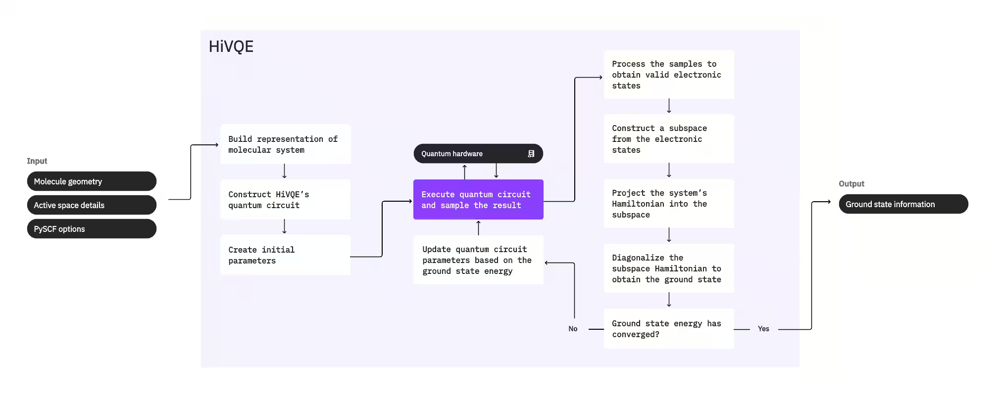
כדי לחשב את מצב היסוד של מערכת, HI-VQE משתמש תחילה בחבילת הכימיה הקלאסית PySCF ליצירת ייצוג מולקולרי מקלטי משתמש, כגון גיאומטריה מולקולרית ומידע מולקולרי אחר. לאחר מכן הוא נכנס ללולאת אופטימיזציה היברידית קוונטית-קלאסית, ומשפר באופן איטרטיבי תת-מרחב כדי לייצג באופן אופטימלי את מצב היסוד תוך מזעור מספר התצורות הכלולות. הלולאה נמשכת עד שמתקיימים קריטריוני התכנסות, כגון גודל תת-מרחב או יציבות אנרגיה, ולאחר מכן פונקציית הגל של מצב היסוד המחושב ואנרגיתו מופקות. ניתן להשתמש בתוצאות אלו לבנייה של עקומות אנרגיה פוטנציאלית מדויקות ולביצוע ניתוח נוסף של המערכת.

לולאת האופטימיזציה מתמקדת בהתאמת פרמטרי Circuit קוונטי ליצירת תת-מרחב איכותי. HI-VQE מציע שלוש אפשרויות Circuit קוונטי: excitation_preserving, efficient_su2, ו-LUCJ. האופטימיזציה מאותחלת קרוב למצב ייחוס Hartree-Fock בשל התאמתו הכללית. ה-Circuit מבוצע לאחר מכן על מכשיר קוונטי ותצורות מדוגמות מהמצב הקוונטי המתקבל לפני שהוחזרו כמחרוזות בינאריות. בשל רעשי מכשיר קוונטי, תצורות מדוגמות מסוימות עשויות להיות פיזיקלית לא חוקיות, ולא לשמר את מספר האלקטרונים או הספין. HI-VQE מטפל בכך באמצעות תהליך שחזור התצורות מחבילת qiskit-addon-sqd, כך שמשתמשים יכולים לתקן תצורות לא חוקיות או להשליך אותן.

לאחר מכן התצורות החוקיות עוברות שלב סינון אופציונלי להסרת אלה שחזויות לתרום באופן מינימלי. זה מפחית את הממד של תת-המרחב, ומוריד בכך את עלות שלב האלכסון. אם הסינון מופעל, נבנה Hamiltonian תת-מרחב ראשוני מהתצורות החוקיות ומבוצע אלכסון עם קריטריוני סיום רופפים מאוד. למרות שדיוק האמפליטודות המתקבלות לכל תצורה נמוך, הוא יעיל לחיזוי אילו תצורות להשאיר מחוץ לתת-המרחב באיטרציה זו, וניתן לחישוב מהיר.

התצורות שנבחרו מתווספות לתת-המרחב, ו-Hamiltonian של המערכת מוקרן לתוך תת-מרחב זה. תת-המרחב מתעדכן באופן איטרטיבי, תוך שמירה על התצורות הרלוונטיות ביותר לאורך איטרציות. גישה זו מנוגדת לשיטות חלופיות מכיוון ש-Circuit הקוונטי אינו צריך לקרב את מצב היסוד המלא בכל שלב.

לאחר מכן, ה-Hamiltonian של תת-המרחב מאולכסן קלאסית לקבלת ערך העצמי הנמוך ביותר ווקטור העצמי המתאים לו, המייצג קירוב של מצב היסוד ואנרגיתו. ככל שאיכות תת-המרחב משתפרת דרך איטרציות, מצב היסוד המחושב מקרב טוב יותר את מצב היסוד האמיתי. ניתן לבצע שלב סינון נוסף בשלב זה להסרת תצורות כלשהן מתת-המרחב שאין להן תרומה משמעותית למצב היסוד המחושב. שלב זה מבטיח שתת-המרחב המועבר לאיטרציה הבאה יהיה קומפקטי ככל האפשר. הדבר מוערך בהתבסס על האמפליטודות שמוחזרות על ידי האלכסון, מכיוון שאלה מייצגות את תרומת החשיבות של כל תצורה למצב היסוד המחושב.

לאחר מכן בדיקת התכנסות קובעת אם אימון נוסף ישפר את התוצאות. אם כן, שלב התרחבות קלאסי אופציונלי מבוצע, פרמטרי Circuit הקוונטי מתעדכנים כדי למזער עוד את האנרגיה המחושבת, והתהליך חוזר. שלב ההתרחבות הקלאסי מייצר תצורות נוספות עבור תת-המרחב, המשלימות את התצורות שנדגמו מהמכשיר הקוונטי. הוא מזהה תחילה את התצורה עם האמפליטודה הגדולה ביותר בתוצאות האלכסון, לפני שמייצר תצורות חדשות עם עירורים בודדים וכפולים מהתצורה שזוהתה. לאחר מכן מספר התצורות הרצוי מאלה מתווסף לתת-המרחב.

לאחר שנקבע שהאיטרציות התכנסו, HI-VQE מחזיר את מצב היסוד המחושב (בצורת המצבים בתת-המרחב ואמפליטודותיהם בפונקציית הגל של מצב היסוד), אנרגיתו, ומדד שונות אנרגיה המעיד אם המצב המחושב מהווה ערך עצמי של ה-Hamiltonian של המערכת.

משתמשים יכולים להחליט על ה-Circuit הקוונטי בשימוש ועל מספר ה-shots שיילקחו לכל Circuit קוונטי, וכן לשלוט בגודל תת-המרחב או לאפשר יצירה קלאסית של תצורות נוספות לסיוע בתצורות שנוצרו קוונטית. בדרך זו משתמשים יכולים להתאים את התנהגות HI-VQE לאפליקציות הרצויות להם.

התחלה

ראשית, בקש גישה לפונקציה. לאחר מכן, אמת את זהותך באמצעות מפתח ה-API של IBM Quantum® ובהנחה שכבר שמרת את חשבונך לסביבה המקומית שלך, בחר את פונקציית Qiskit כך:

import reprlib
from qiskit_ibm_catalog import QiskitFunctionsCatalog

catalog = QiskitFunctionsCatalog(channel="ibm_quantum_platform")

function = catalog.load("qunova/hivqe-chemistry")

קלטים

ראה את הטבלה הבאה לכל פרמטרי הקלט שהפונקציה מקבלת. הסעיפים הבאים אפשרויות מולקולה ו-אפשרויות HI-VQE מפרטים יותר על הארגומנטים הללו.

Name	Type	Description	Required	Default	Example
geometry	Union[List[List[Union[str, Tuple[float, float, float]]]], str]	This can be either a string or structured lists containing atom and coordinate pairs. If this is given as a string, it must be a molecule geometry in Cartesian Coordinate Format. If this is given as a list, it should be given as a list of lists that each contain an atom string and coordinate tuple.	Yes	N/A	[['O', (0, 0, 0)], ['H', (0, 1, 0)], ['H', (0, 0, 1)]] or "O 0 0 0; H 0 1 0; H 0 0 1"
backend_name	str	Name of the backend to make the query.	Yes	N/A	ibm_fez
max_states	int	The maximum subspace dimension for the diagonalization. Fewer states will be used if the number is not a perfect square.	Yes	N/A	100
max_expansion_states	int	The maximum number of classically-generated CI states to be included in each iteration.	Yes	N/A	10
molecule_options	dict	Options related to the molecule used as input to HI-VQE. See the Molecule options section for more details.	No	See the Molecule options section for details.	{"basis": "sto3g", "unit": "angstrom" }
hivqe_options	dict	Options controlling the behavior of the HI-VQE algorithm. See the HI-VQE options section for more details.	No	See the HI-VQE options section for details.	{"shots": 10_000, "max_iter": 10 }

אפשרויות מולקולה

הטבלה הבאה מפרטת את כל המפתחות והערכים שניתן להגדיר במילון molecule_options, כמו גם סוגי הנתונים וערכי ברירת המחדל שלהם. כל המפתחות אופציונליים.

Key	Value type	Default Value	Valid range	Explanation
"charge"	int	0	Various	An integer specifying the total net charge of the molecular system. The default value is 0; however, it can be any integer.
"basis"	str	'sto-3g'	Various	A string specifying the basis type; these are passed to pyscf. (eg: "sto-3g", "3-21g", "6-31g", "cc-pvdz")
"active_orbitals"	List[int]	Every orbital index.	The spatial orbital indices valid for the problem.	A list of active orbital indices in the interval [0, n) where n is the number of qubits used in the problem. If this is specified, then the frozen_orbitals argument must also be specified.
"frozen_orbitals"	List[int]	No indices.	The spatial orbital indices valid for the problem, excluding active orbitals.	A list of frozen orbital indices in the same range as active_orbitals. If specified, then active_orbitals must also be specified. Note that only occupied orbitals should be frozen as the number of active electrons is reduced by 2 for every occupied orbital that is frozen.
"orbital_coeffs"	List[List[float]]	Hartree-Fock molecular orbitals.	Various.	The coefficients for the spatial orbitals used in the calculation of the electronic repulsion integrals for the system. Some valid examples are Hartree-Fock molecular orbitals, natural orbitals, and AVAS orbitals.
"symmetry"	Union[str, bool]	False	True or False	Used to invoke point group symmetry for the initial molecular calculations to construct the symmetry adapted orbital basis. These symmetry-adapted orbitals are used as basis functions for the following SCF calculations. The default value is False; if set to True, then it will be invoked and arbitrary point groups will automatically be detected and used. If a particular symmetry is assigned, for example, symmetry = "Dooh", then an error will be raised if the molecular geometry is not subject to this required symmetry.
"symmetry_subgroup"	Optional[str]	None	See pyscf documentation.	Can be used to generate a subgroup of the detected symmetry. This has no effect when symmetry is specified using the symmetry keyword argument.
"unit"	str	"angstrom"	See pyscf documentation.	Specifies the measurement unit to use for atomic coordinates and distances. The default is to use angstrom units.
"nucmod"	Optional[Union[dict, str]]	None	See pyscf documentation.	Specifies the nuclear model to be used. By default it uses the point nuclear model, and other values enable Gaussian nuclear model. If a function is given, it will be used with the Gaussian nuclear model to generate the nuclear charge distribution value 'zeta'.
"pseudo"	Optional[Union[dict, str]]	None	See pyscf documentation.	Specifies the pseudopotential for the atoms in the molecule. This is None by default, indicating that no pseudopotentials are applied and all electrons are explicitly included in the calculations.
"cart"	bool	False	See pyscf documentation.	Specifies whether to use cartesian GTOs as the angular momentum basis functions in the calculation. The default value of False will use spherical GTOs.
"magmom"	Optional[List[Union[int, float]]]	None	See pyscf documentation.	Sets the colinear spin magnetic moment of each atom. By default, this is None and each atom is initialized with a spin of zero.
"avas_aolabels"	Optional[List[str]]	None	i.e. ["H 1s", "O 2p"] for H2O	This defines Atomic Orbital to be included in AVAS scheme. See AVAS documentation .
"avas_threshold"	float	0.2	Between 0.0 and 2.0	This specifies the cutoff value used to determine which Atomic Orbitals (AOs) are retained in the active space.
"noons_level"	Optional[str]	None	"mp2" or "ccsd"	This defines the theoretical approach for preparing natural orbitals and selecting active orbitals based on the Natural Orbital Occupation Numbers (NOONs) scheme. See NOONs documentation. Both the active and frozen orbital indices must be provided to control the number of orbitals (and the number of qubits).

אפשרויות HI-VQE

הטבלה הבאה מפרטת את כל המפתחות והערכים שניתן להגדיר במילון hivqe_options, כמו גם סוגי הנתונים וערכי ברירת המחדל שלהם. כל המפתחות אופציונליים.

Key	Value type	Default Value	Valid range	Explanation
"shots"	int	1_000	Between 1 and 10 000.	Number of shots to use on the quantum device per iteration.
"max_iter"	int	25	Between 1 and 50.	The maximum number of iterations to run to optimize the ansatz. The algorithm may use fewer iterations if convergence is achieved early.
"initial_basis_states"	List[str]	The Hartree-Fock state.	Binary strings with the number of bits matching the required number of qubits for the problem.	Can be used to restart the algorithm with classical states from a previous result.
"ansatz"	str	"epa"	"epa", "hea", or "lucj"	This specifies the quantum ansatz to optimize to generate new states. "epa" selects the excitation-preserving ansatz. "hea" selects the hardware-efficient ansatz. "lucj" selects the local unitary cluster Jastrow ansatz.
"convergence_count"	int	3	At least 2.	The number of iterations without significant change of the computed energy that should elapse before the algorithm is deemed to have converged.
"convergence_abstol"	float	1e-4	More than 0 and at most 1.	The magnitude of change in computed energy that is considered significant for the purposes of convergence checks.
"reset_convergence_count"	bool	True	True or False	If True, the convergence_count iterations must occur without an interrupting significant change to qualify as converging. If False, then the algorithm will stop after convergence_count if insignificant changes have occurred at any iterations during the optimization process.
"configuration_recovery"	bool	True	True or False.	Whether or not to use configuration recovery from the qiskit-addon-sqd package. If True, invalid states sampled from the quantum device are corrected classically. If False, they are discarded.
"ansatz_entanglement"	str	"circular"	Any one of "linear", "reverse_linear", "pairwise", "circular", "full", or "sca". If using the "lucj" ansatz, "lucj_default" is also an option.	This specifies the entanglement scheme that should be used within the quantum circuit, following common Qiskit and ffsim conventions for the LUCJ ansatz.
"ansatz_reps"	int	2	Greater than 0.	The number of repetitions of each layer in the quantum circuit.
"amplitude_screening_tolerance"	Union[float,int]	0	At least 0, and less than 1.	The tolerance for deciding which states should be screened out of the subspace after diagonalization. It specifies the inclusion threshold for the subspace states based on their computed amplitudes.
"overlap_screening_tolerance"	float	1e-2	Between 1e-4 and 1e-1, inclusive.	The tolerance for predicting which states should be screened out of the subspace prior to diagonalization. It controls the accuracy of the predicted amplitudes for each state, with a smaller value resulting in more accurate predictions.

פלטים

הפונקציה מחזירה מילון עם ארבעה מפתחות וערכים. המפתחות והערכים מתועדים בטבלה הבאה:

Key	Value Type	Explanation
"energy"	float	The approximate ground state energy of the molecule.
"states"	List[str]	The selected determinants that form the subspace used to solve for the energy. They are in alternating alpha-beta format.
"eigenvector"	List[float]	The eigenvector corresponding to the ground state of the subspace composed of "states".
"energy_variance"	float	The energy variance of the ground state of the subspace composed of "states", giving an indication of the quality of the solution. This value is non-negative and a lower value means that the ground state of the subspace more closely approximates an eigenstate of the system's Hamiltonian.
"energy_history"	List[float]	The energies computed each iteration during the hybrid optimization process, in the same order that they were computed. Two energies are computed per iteration as part of the SPSA optimization process.

דוגמה

הדוגמה הראשונה מראה כיצד לחשב את אנרגיית מצב היסוד עבור מולקולת NH3 באמצעות אלגוריתם HI-VQE.

הגדר את הגיאומטריה המולקולרית והאפשרויות

הגיאומטריה המולקולרית של NH3 מסופקת עם קואורדינטות קרטזיות מופרדות ב-";" לכל אטום.

# Define the molecule geometry
geometry = """
N         -0.85188       -0.02741        0.03141;
H          0.16545        0.00593       -0.01648;
H         -1.16348       -0.39357       -0.86702;
H         -1.16348        0.94228        0.06281;
"""

ניתן להגדיר ולספק אפשרויות נוספות עבור המערכת המולקולרית בפורמט מילון הבא.

# Configure some options for the job.
molecule_options = {"basis": "sto3g"}
hivqe_options = {"shots": 100, "max_iter": 20}

הרץ את הפונקציה עם קלטי הגיאומטריה והאפשרויות.

# Run HI-VQE
job = function.run(
    geometry=geometry,
    # `backend_name` is the name of a backend with at least 16 qubits, for example, "ibm_marrakesh".
    backend_name=backend_name,
    max_states=2000,
    max_expansion_states=10,
    molecule_options=molecule_options,
    hivqe_options=hivqe_options,
)

כדאי להדפיס את מזהה עבודת הפונקציה כדי שיהיה ניתן לספקו בבקשות תמיכה אם משהו משתבש.

print("Job ID:", job.job_id)

Job ID: 128ee399-7cfc-4be2-91e9-c4abd22b97c7

דוגמה זו משתמשת אז ב-16 Qubit עם 8 אורביטלים של בסיס sto3g עבור מולקולת NH3. בדוק את הסטטוס של עומס עבודה Qiskit Function שלך או קבל תוצאות כך:

print(job.status())

QUEUED

לאחר השלמת העבודה, ניתן לקבל את התוצאות עם מופע result().

result = job.result()

# Output can be long, so we display a shortened representation
shortened_result = reprlib.repr(result)
print(shortened_result)

{'eigenvector': [0.9824200343205695, 0.009520846167419264, 6.365368845740147e-08, 3.6832123006425615e-07, 0.0012869941182066654, 2.3403891050875465e-05, ...], 'energy': -55.521146537970466, 'energy_history': [-55.52091922342852, -55.52113695367561, -55.521146537970466, -55.52114653864798, -55.521146537970466, -55.521146537970466, ...], 'energy_variance': 9.788555455342562e-12, ...}

כדי לגשת לאנרגיית מצב היסוד, השתמש במפתח "energy". המפתח "eigenvector" מספק את מקדמי ה-CI עם סימון מחרוזת סיביות מתאים של תצורת אלקטרונים המאוחסן עם "states" של התוצאות.

fci_energy = -55.521148034704126  # the exact energy using FCI method
hivqe_energy = result["energy"]
print(
    f"|Exact Energy - HI-VQE Energy|: {abs(fci_energy - hivqe_energy) * 1000} mHa"
)
print(f"Sampled Number of States: {len(result['states'])}")

|Exact Energy - HI-VQE Energy|: 0.0014967336596782843 mHa
Sampled Number of States: 1936

פלט:

|Exact Energy - HI-VQE Energy|: 0.077237504 mHa Sampled Number of States: 1936

ביצועים

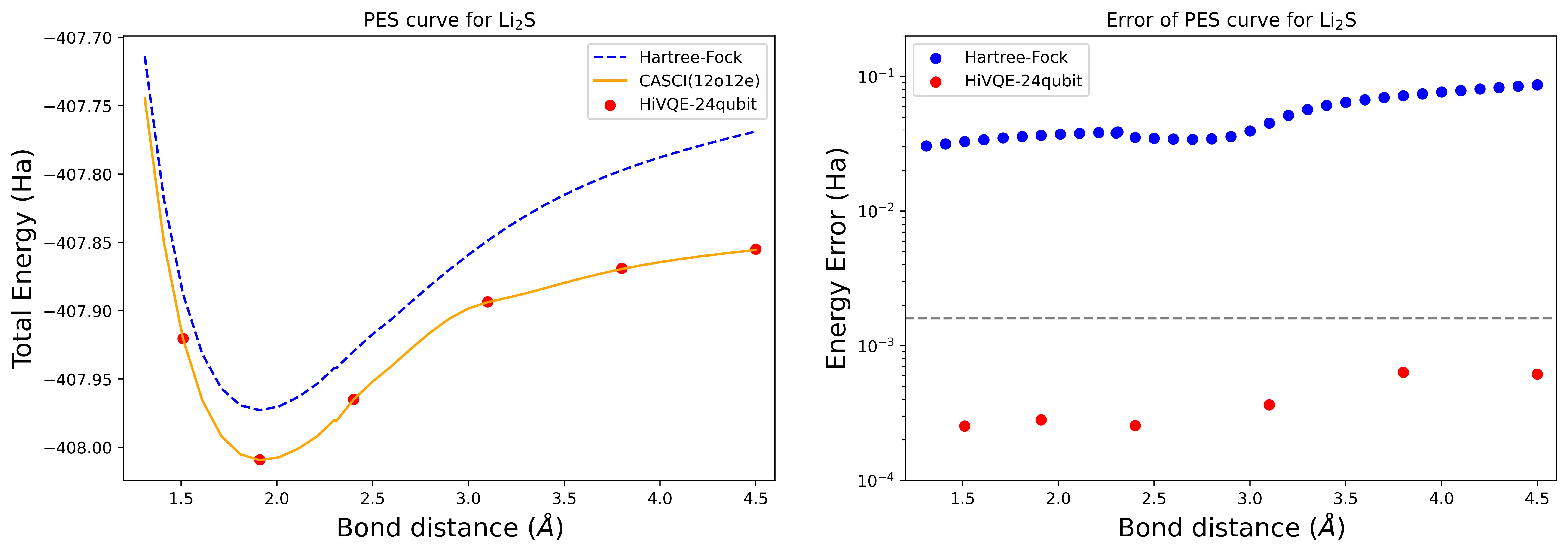
חלק זה מציג חישובי benchmark מוכחים של HI-VQE עבור מקרה של 24 Qubit עבור Li2S, מקרה של 40 Qubit עבור מולקולת N2, ומקרה של 44 Qubit עבור מערכת FeP-NO.

עקומת מישטח אנרגיה פוטנציאלי (PES) לניתוק מולקולת Li2S עם 24 Qubit

עקומת PES מוצגת עם ייחוס FCI וניחוש ראשוני מ-RHF, יחד עם שגיאת האנרגיה מייחוס FCI.

החישובים בוצעו עם הגיאומטריות והאפשרויות הבאות.

# This cell is hidden from users
backend_name = service.least_busy(operational=True, min_num_qubits=38).name

# Define Li2S geometries
Li2S_geoms = {
    "Li2S_1.51": "S        -1.239044    0.671232   -0.030374;Li       -1.506327    0.432403   -1.498949;Li       -0.899996    0.973348    1.826768;",
    "Li2S_2.40": "S        -1.741432    0.680397    0.346702;Li       -0.529307    0.488006   -1.729343;Li       -1.284307    0.989409    2.177209;",
    "Li2S_3.80": "S        -2.707255    0.674298    0.909161;Li        0.079218    0.552012   -1.671656;Li       -0.927010    0.931502    1.557063;",
}

# Configure some options for the job.
molecule_options = {
    "basis": "sto3g",
}
hivqe_options = {
    "shots": 100,
    "max_iter": 20,
}

results = []
for geom in ["Li2S_1.51", "Li2S_2.40", "Li2S_3.80"]:
    # Run HI-VQE
    job = function.run(
        geometry=Li2S_geoms[geom],
        backend_name=backend_name,  # can use any device with at least 38 qubits
        max_states=2000,
        max_expansion_states=10,
        molecule_options=molecule_options,
        hivqe_options=hivqe_options,
    )
    results.append(job.result())

הנקודות האדומות מייצגות את תוצאות חישוב HI-VQE עבור שש גיאומטריות שונות, ושלוש גיאומטריות המתאימות ל-1.51, 2.40, ו-3.80 אנגסטרום מסופקות כקלט בתא לעיל.

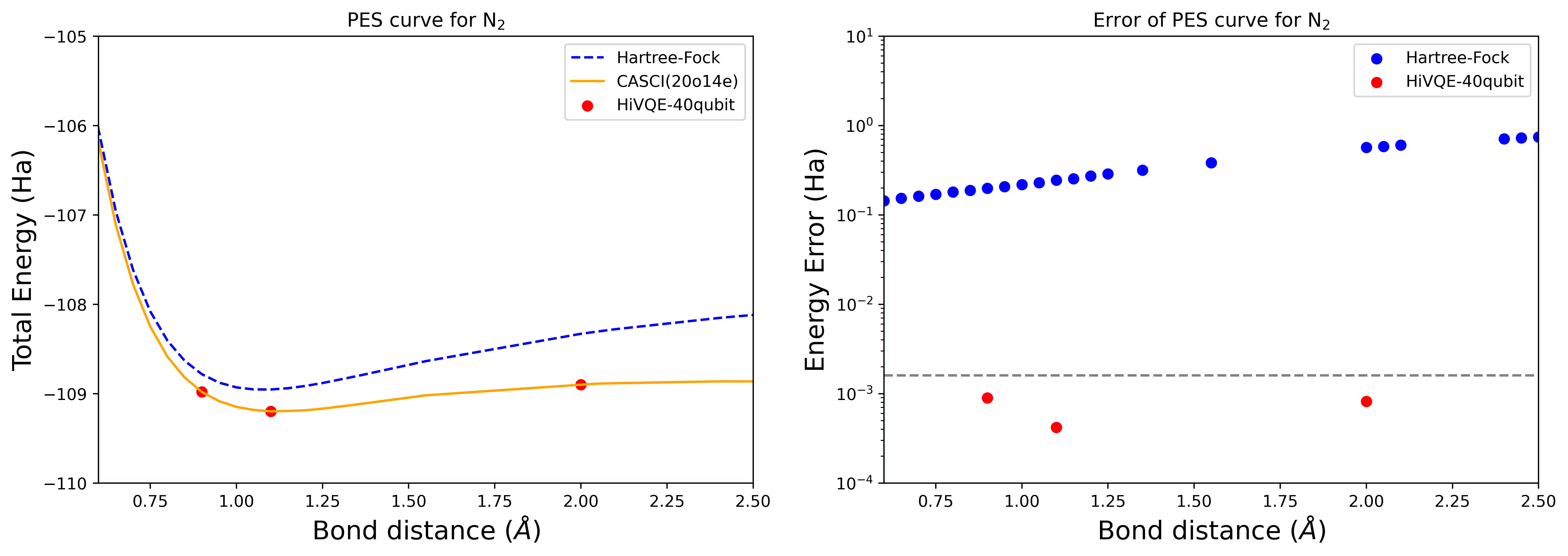
עקומת PES לניתוק עבור מולקולת N2 עם 40 Qubit

מולקולת החנקן זוהתה כמערכת multireference עם תרומות אנרגיה קורלציה גדולות מעבר למצב Hartree-Fock. ביצענו חישוב benchmark עבור מולקולת N2 עם בסיס cc-pvdz, (20o,14e) באמצעות בחירת אורביטל פעיל homo-lumo. מספר המרחב הפעיל המלא (CAS) לייצוג בעיה זו הוא 6,009,350,400. אין אפשרות לקבל את פתרון בעיית הערכים העצמיים (עבור אנרגיה ומבנה אלקטרוני) עם מספר מצבים זה באמצעות מחשב שולחני רב-עוצמה (16cpu/64GB). עם HI-VQE, משתמשים יכולים לחפש ביעילות את תת-המרחב של מצבי CAS למציאת תוצאות מדויקות כימית תוך חיסכון משמעותי במשאבי חישוב. הגרפים הבאים מראים את עקומת PES של חישוב HI-VQE בן 40 Qubit של ניתוק מולקולת N2.

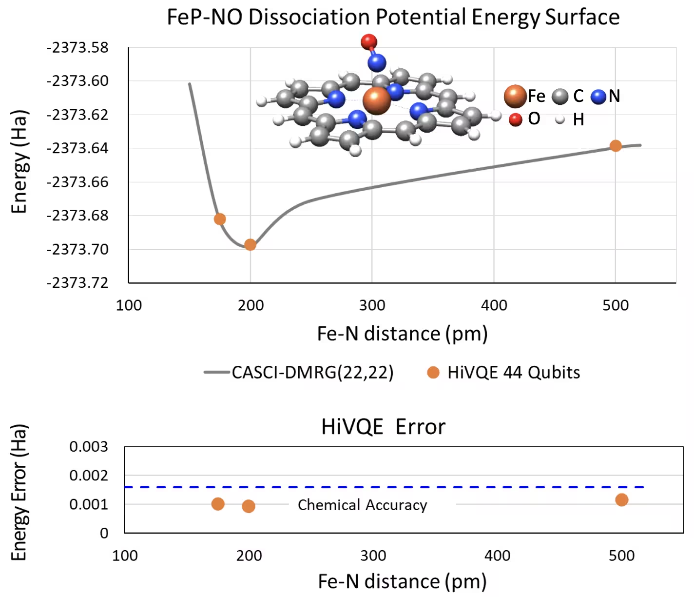
עקומת PES לניתוק עבור ברזל(II)-פורפירין חמישה-מתואם עם מערכת NO עם 44 Qubit

מערכת כימית מעניינת נוספת היא קומפלקס ברזל(II)-פורפירין (FeP) עם ליגנד תחמוצת חנקן (NO) מתואם, המייצג מערכת מטלופורפירין רלוונטית ביולוגית הממלאת תפקידים מכריעים בתהליכים פיזיולוגיים שונים. בדוגמה זו, נעשה שימוש ב-HI-VQE להערכת עקומת מישטח אנרגיה פוטנציאלי מדויקת של האינטראקציה הבין-מולקולרית בין FeP ל-NO (אנרגיית מצב היסוד עבור גיאומטריות מופרדות באופן שונה). למערכת המשולבת יש 450 אורביטלים ו-202 אלקטרונים (450o,202e) עם בסיס 6-31g(d) בסך הכל. בחירת אורביטל פעיל homo-lumo שימשה לחישוב המקרה הקטן יותר מהמקרה האמיתי עם (22o,22e). מתוצאות ה-benchmark הבאות, הצלחנו להשיג דיוק כימי (> 1.6 mHa) עם חישוב כימיה קלאסי מתקדם של ייחוס CASCI(DMRG) (22o,22e).

מדדי ביצועים

• גודל המטריצה המדויק הוא מספר הדטרמיננטים לפתרון מדויק, כגון FCI ו-CASCI.
• HI-VQE מדגם ומחשב את תת-המרחב שלו (כלומר, גודל מטריצת HI-VQE).
• הזמן הכולל כולל זמן ריצת QPU ומופעי Qiskit Function עם CPU.
• הדיוק מוערך מהפרש האנרגיה מהפתרון המדויק.

Chemical system	Number of qubits	Exact matrix size	HI-VQE matrix size	E(diff) from exact (mHa)	Number of iteration	Total time	QPU runtime usage
$NH_3$ (8o,10e)	16	3136	1936	0.08	6	37 s	34 s
$Li_2S$ (10o,10e)	20	63504	3969	0.60	5	250 s	50 s
$NH_3$ (15o,10e)	30	9018009	49729	0.90	5	354 s	54 s
$N_2$ (16o,14e)	32	130873600	1798281	1.10	9	6531 s	121 s
$3H_2O$ (18o,24e)	36	344622096	399424	0.90	24	5174 s	130 s
$N_2$ (20o,14e)	40	6009350400	9012004	1.20	21	46547 s	258 s

אחזור הודעות שגיאה

אם עומס העבודה שלך נכשל, הסטטוס יהיה ERROR וקריאה ל-job.result() תעלה חריגה:

job = function.run(
    geometry="invalid-geometry",  # This will cause an error
    backend_name=backend_name,
    max_states=2000,
    max_expansion_states=15,
    molecule_options=molecule_options,
    hivqe_options=hivqe_options,
)

job.result()

job.status()

'ERROR'

קבלת תמיכה

תוכל לשלוח אימייל ל-qiskit.support@qunovacomputing.com לקבלת עזרה בפונקציה זו.

אם אתה זקוק לעזרה בפתרון שגיאה ספציפית, אנא ספק את מזהה עבודת הפונקציה של העבודה שנתקלה בשגיאה.

הצעדים הבאים

המלצות

• בקש גישה לפונקציה על ידי מילוי טופס זה.
• נסה את המדריך חישוב עקומת PES לניתוק עבור FeP-NO עם HI-VQE.
• עיין ב-Pellow-Jarman, A., et al. (2025). HIVQE: Handover Iterative Variational Quantum Eigensolver for Efficient Quantum Chemistry Calculations. arXiv preprint arXiv:2503.06292.
• נסה את המדריך עקומות PES לניתוק עם Qunova HiVQE.