ליכסון קוונטי Krylov מבוסס-דגימה של מודל סריג פרמיוני
הערכת שימוש: תשע שניות על מעבד Heron r2 (הערה: זוהי הערכה בלבד. זמן הריצה שלך עשוי להשתנות.)
תוצאות למידה
-
כיצד להשתמש ב-SQD Qiskit addon כדי לקרב את אנרגיית מצב היסוד של מודל סריג באמצעות מחרוזות ביטים שנדגמו מיחידת עיבוד קוונטית (QPU).
-
כיצד להשתמש ב-ffsim כדי לבנות מעגלי אבולוציית זמן לסימולציה פרמיונית.
-
כיצד לשלב דגימות ממספר מעגלים לעיבוד-המשך (post-processing) עם אלגוריתם הליכסון Krylov מבוסס-דגימה (SKQD).
דרישות מקדימות
רקע
מדריך זה מראה כיצד להשתמש בליכסון קוונטי מבוסס-דגימה (SQD) כדי להעריך את אנרגיית מצב היסוד של מודל סריג פרמיוני. באופן ספציפי, אנחנו חוקרים את מודל Anderson חד-ממדי עם זיהום בודד (SIAM), המשמש לתיאור זיהומים מגנטיים המוטמעים במתכות.
מדריך זה עוקב אחר תהליך עבודה דומה למדריך הקשור ליכסון קוונטי מבוסס-דגימה של המילטוניאן כימי. עם זאת, הבדל מרכזי טמון באופן בו המעגלים הקוונטיים נבנים. המדריך האחר משתמש ב-ansatz וריאציוני היוריסטי, שמתאים להמילטוניאנים כימיים שעשויים לכלול מיליוני מונחי אינטראקציה. מצד שני, מדריך זה משתמש במעגלים המקרבים אבולוציית זמן על ידי ההמילטוניאן. מעגלים כאלה יכולים להיות עמוקים, ולכן גישה זו מתאימה יותר ליישומים למודלי סריג. וקטורי המצב המוכנים על ידי מעגלים אלה מהווים את הבסיס ל-תת-מרחב Krylov, וכתוצאה מכך, האלגוריתם מתכנס באופן מוכח ויעיל למצב היסוד, בהנחות מתאימות.
את הגישה המשמשת במדריך זה ניתן לראות כשילוב של הטכניקות המשמשות ב-SQD ו-ליכסון קוונטי Krylov (KQD). הגישה המשולבת מכונה לעתים ליכסון קוונטי Krylov מבוסס-דגימה (SQKD). ראה ליכסון קוונטי Krylov של המילטוניאני סריג למדריך על שיטת KQD.
מדריך זה מבוסס על העבודה "Quantum-Centric Algorithm for Sample-Based Krylov Diagonalization", שאליה ניתן לפנות לפרטים נוספים.
מודל Anderson עם זיהום בודד (SIAM)
ההמילטוניאן חד-ממדי SIAM הוא סכום של שלושה מונחים:
כאשר
כאן, הם אופרטורי היצירה/ההשמדה הפרמיוניים עבור אתר האמבט ה- עם ספין , הם אופרטורי יצירה/השמדה עבור מוד הזיהום, ו-. , , ו- הם מספרים ממשיים המתארים את האינטראקציות של דילוג, באתר והיברידיזציה, ו- הוא מספר ממשי המציין את הפוטנציאל הכימי.
שים לב שההמילטוניאן הוא מופע ספציפי של ההמילטוניאן הגנרי של אלקטרון-אינטראקציה,
כאשר מורכב ממונחי גוף-אחד, שהם ריבועיים באופרטורי היצירה וההשמדה הפרמיוניים, ו- מורכב ממונחי שני-גופים, שהם רביעיים. עבור SIAM,
ו- מכיל את שאר המונחים בהמילטוניאן. כדי לייצג את ההמילטוניאן באופן תוכניתי, אנחנו מאחסנים את המטריצה ואת הטנזור .
בסיסי מיקום ותנע
בשל הסימטריה הטרנסלציונית המקורבת ב-, אנחנו לא מצפים שמצב היסוד יהיה דליל בבסיס המיקום (בסיס האורביטלים שבו ההמילטוניאן מוגדר למעלה). הביצועים של SQD מובטחים רק אם מצב היסוד דליל, כלומר, יש לו משקל משמעותי רק על מספר קטן של מצבי בסיס חישוביים. כדי לשפר את הדלילות של מצב היסוד, אנחנו מבצעים את הסימולציה בבסיס האורביטלים שבו הוא אלכסוני. אנחנו קוראים לבסיס זה בסיס תנע. מכיוון ש- הוא המילטוניאן פרמיוני ריבועי, ניתן לאלכסן אותו ביעילות על ידי סיבוב אורביטלי.
קירוב אבולוציית זמן על ידי ההמילטוניאן
כדי לקרב אבולוציית זמן על ידי ההמילטוניאן, אנחנו משתמשים בפירוק Trotter-Suzuki מסדר שני,
תחת טרנספורמציית Jordan-Wigner, אבולוציית זמן על ידי מסתכמת בשער CPhase בודד בין האורביטלים ספין-למעלה וספין-למטה באתר הזיהום. מכיוון ש- הוא המילטוניאן פרמיוני ריבועי, אבולוציית זמן על ידי מסתכמת בסיבוב אורביטלי.
מצבי בסיס Krylov , כאשר הוא הממד של תת-מרחב Krylov, נוצרים על ידי יישום חוזר של צעד Trotter בודד, כך ש
בתהליך העבודה המבוסס-SQD הבא, נדגום מקבוצת המעגלים הזו ונבצע עיבוד-המשך (post-processing) לקבוצת מחרוזות הביטים המשולבת באמצעות SQD. גישה זו שונה מזו המשמשת במדריך הקשור ליכסון קוונטי מבוסס-דגימה של המילטוניאן כימי, שבו דגימות נלקחו ממעגל וריאציוני היוריסטי בודד.
דרישות
לפני שתתחיל במדריך זה, ודא שיש לך את הדברים הבאים מותקנים:
-
Qiskit SDK v1.0 או מאוחר יותר, עם תמיכת visualization
-
Qiskit Runtime v0.22 או מאוחר יותר (
pip install qiskit-ibm-runtime) -
SQD Qiskit addon v0.11 או מאוחר יותר (
pip install qiskit-addon-sqd) -
ffsim v0.0.72 או מאוחר יותר (
pip install ffsim)
דוגמת סימולטור בקנה מידה קטן
שלב 1: מיפוי בעיה למעגל קוונטי
ראשית, אנחנו מייצרים את ההמילטוניאן SIAM בבסיס המיקום. ההמילטוניאן מיוצג על ידי המטריצה והטנזור . לאחר מכן, אנחנו מסובבים אותו לבסיס התנע. בבסיס המיקום, אנחנו ממקמים את הזיהום באתר הראשון. עם זאת, כאשר אנחנו מסובבים לבסיס התנע, אנחנו מעבירים את הזיהום לאתר מרכזי כדי להקל על אינטראקציות עם אורביטלים אחרים.
# Added by doQumentation — installs the packages this notebook needs if they are missing
import importlib.util

_needed = {"ffsim": "ffsim", "matplotlib": "matplotlib", "numpy": "numpy", "pyscf": "pyscf", "qiskit": "qiskit", "qiskit_addon_sqd": "qiskit-addon-sqd", "qiskit_ibm_runtime": "qiskit-ibm-runtime", "scipy": "scipy"}
_missing = [pip for module, pip in _needed.items()
            if importlib.util.find_spec(module) is None]
# One at a time, so a package that fails to install does not block the others
for _pip in _missing:
    %pip install -q {_pip}
if not _missing:
    print("\u2713 All required packages are installed")
import numpy as np
import pyscf.fci

def siam_hamiltonian(
    norb: int,
    hopping: float,
    onsite: float,
    hybridization: float,
    chemical_potential: float,
) -> tuple[np.ndarray, np.ndarray]:
    """Hamiltonian for the single-impurity Anderson model."""
    # Place the impurity on the first site
    impurity_orb = 0

    # One body matrix elements in the "position" basis
    h1e = np.zeros((norb, norb))
    np.fill_diagonal(h1e[:, 1:], -hopping)
    np.fill_diagonal(h1e[1:, :], -hopping)
    h1e[impurity_orb, impurity_orb + 1] = -hybridization
    h1e[impurity_orb + 1, impurity_orb] = -hybridization
    h1e[impurity_orb, impurity_orb] = chemical_potential

    # Two body matrix elements in the "position" basis
    h2e = np.zeros((norb, norb, norb, norb))
    h2e[impurity_orb, impurity_orb, impurity_orb, impurity_orb] = onsite

    return h1e, h2e

def momentum_basis(norb: int) -> np.ndarray:
    """Get the orbital rotation to change from the position to the momentum basis."""
    n_bath = norb - 1

    # Orbital rotation that diagonalizes the bath (non-interacting system)
    hopping_matrix = np.zeros((n_bath, n_bath))
    np.fill_diagonal(hopping_matrix[:, 1:], -1)
    np.fill_diagonal(hopping_matrix[1:, :], -1)
    _, vecs = np.linalg.eigh(hopping_matrix)

    # Expand to include impurity
    orbital_rotation = np.zeros((norb, norb))
    # Impurity is on the first site
    orbital_rotation[0, 0] = 1
    orbital_rotation[1:, 1:] = vecs

    # Move the impurity to the center
    new_index = n_bath // 2
    perm = np.r_[1 : (new_index + 1), 0, (new_index + 1) : norb]
    orbital_rotation = orbital_rotation[:, perm]

    return orbital_rotation

def rotated(
    h1e: np.ndarray, h2e: np.ndarray, orbital_rotation: np.ndarray
) -> tuple[np.ndarray, np.ndarray]:
    """Rotate the orbital basis of a Hamiltonian."""
    h1e_rotated = np.einsum(
        "ab,Aa,Bb->AB",
        h1e,
        orbital_rotation,
        orbital_rotation.conj(),
        optimize="greedy",
    )
    h2e_rotated = np.einsum(
        "abcd,Aa,Bb,Cc,Dd->ABCD",
        h2e,
        orbital_rotation,
        orbital_rotation.conj(),
        orbital_rotation,
        orbital_rotation.conj(),
        optimize="greedy",
    )
    return h1e_rotated, h2e_rotated

# Total number of spatial orbitals, including the bath sites and the impurity
# This should be an even number
norb = 8

# System is half-filled
nelec = (norb // 2, norb // 2)
# One orbital is the impurity, the rest are bath sites
n_bath = norb - 1

# Hamiltonian parameters
hybridization = 1.0
hopping = 1.0
onsite = 10.0
chemical_potential = -0.5 * onsite

# Generate Hamiltonian in position basis
h1e, h2e = siam_hamiltonian(
    norb=norb,
    hopping=hopping,
    onsite=onsite,
    hybridization=hybridization,
    chemical_potential=chemical_potential,
)

# Rotate to momentum basis
orbital_rotation = momentum_basis(norb)
h1e_momentum, h2e_momentum = rotated(h1e, h2e, orbital_rotation.T.conj())
# In the momentum basis, the impurity is placed in the center
impurity_index = n_bath // 2

# Use PySCF to compute the exact ground state energy
reference_energy, _ = pyscf.fci.direct_spin1.kernel(h1e, h2e, norb, nelec)
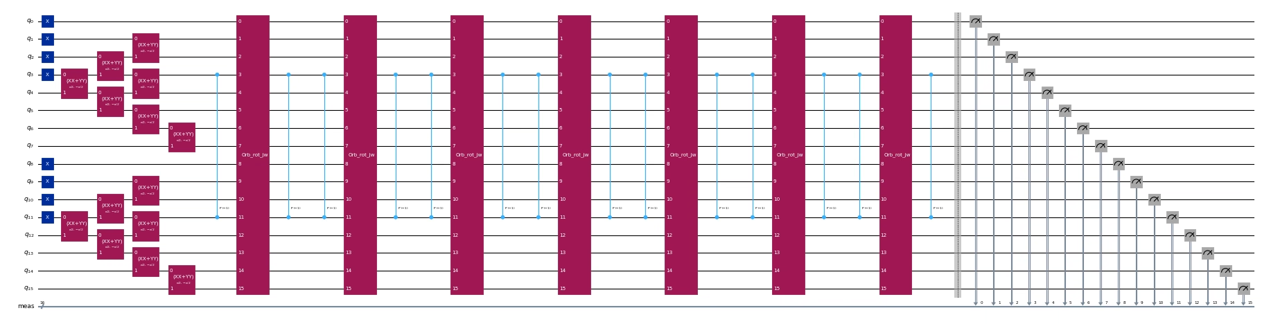
לאחר מכן, אנחנו מייצרים את המעגלים לייצור מצבי בסיס Krylov. עבור כל מין ספין, המצב ההתחלתי ניתן על ידי סופרפוזיציה של כל העירורים האפשריים של שלושת האלקטרונים הקרובים ביותר לרמת Fermi לתוך 4 המודים הריקים הקרובים ביותר החל מהמצב , ומומש על ידי יישום שבעה XXPlusYYGates. המצבים שעברו אבולוציית זמן מיוצרים על ידי יישומים עוקבים של צעד Trotter מסדר שני.
לתיאור מפורט יותר של מודל זה וכיצד המעגלים מתוכננים, ראה ב-"Quantum-Centric Algorithm for Sample-Based Krylov Diagonalization".
from typing import Sequence

import ffsim
import scipy
from qiskit import QuantumCircuit, QuantumRegister
from qiskit.circuit import CircuitInstruction, Qubit
from qiskit.circuit.library import CPhaseGate, XGate, XXPlusYYGate

def prepare_initial_state(qubits: Sequence[Qubit], norb: int, nocc: int):
    """Prepare initial state."""
    assert norb >= 8
    x_gate = XGate()
    rot = XXPlusYYGate(0.5 * np.pi, -0.5 * np.pi)
    for i in range(nocc):
        yield CircuitInstruction(x_gate, [qubits[i]])
        yield CircuitInstruction(x_gate, [qubits[norb + i]])
    for i in range(3):
        for j in range(nocc - i - 1, nocc + i, 2):
            yield CircuitInstruction(rot, [qubits[j], qubits[j + 1]])
            yield CircuitInstruction(
                rot, [qubits[norb + j], qubits[norb + j + 1]]
            )
    yield CircuitInstruction(rot, [qubits[j + 1], qubits[j + 2]])
    yield CircuitInstruction(
        rot, [qubits[norb + j + 1], qubits[norb + j + 2]]
    )

def trotter_step(
    qubits: Sequence[Qubit],
    time_step: float,
    one_body_evolution: np.ndarray,
    h2e: np.ndarray,
    impurity_index: int,
    norb: int,
):
    """A Trotter step."""
    # Assume the two-body interaction is just the on-site interaction of the impurity
    onsite = h2e[
        impurity_index, impurity_index, impurity_index, impurity_index
    ]
    # Two-body evolution for half the time
    yield CircuitInstruction(
        CPhaseGate(-0.5 * time_step * onsite),
        [qubits[impurity_index], qubits[norb + impurity_index]],
    )
    # One-body evolution for the full time
    yield CircuitInstruction(
        ffsim.qiskit.OrbitalRotationJW(norb, one_body_evolution), qubits
    )
    # Two-body evolution for half the time
    yield CircuitInstruction(
        CPhaseGate(-0.5 * time_step * onsite),
        [qubits[impurity_index], qubits[norb + impurity_index]],
    )

# Time step
time_step = 0.2
# Number of Krylov basis states
krylov_dim = 8

# Initialize circuit
qubits = QuantumRegister(2 * norb, name="q")
circuit = QuantumCircuit(qubits)

# Generate initial state
for instruction in prepare_initial_state(qubits, norb=norb, nocc=norb // 2):
    circuit.append(instruction)
circuit.measure_all()

# Create list of circuits, starting with the initial state circuit
circuits = [circuit.copy()]

# Add time evolution circuits to the list
one_body_evolution = scipy.linalg.expm(-1j * time_step * h1e_momentum)
for i in range(krylov_dim - 1):
    # Remove measurements
    circuit.remove_final_measurements()
    # Append another Trotter step
    for instruction in trotter_step(
        qubits,
        time_step,
        one_body_evolution,
        h2e_momentum,
        impurity_index,
        norb,
    ):
        circuit.append(instruction)
    # Measure qubits
    circuit.measure_all()
    # Add a copy of the circuit to the list
    circuits.append(circuit.copy())
circuits[0].draw("mpl", scale=0.4, fold=-1)

circuits[-1].draw("mpl", scale=0.4, fold=-1)
שלב 2: אופטימיזציה של הבעיה להרצה קוונטית
כעת, אנחנו מבצעים אופטימיזציה של המעגל עבור חומרת יעד. לעת עתה, נייצר backend גנרי עם מספר קיוביטים מוגדר וסט שערים שמעגלי אבולוציית הזמן מתפרקים אליהם באופן טבעי.
from qiskit.providers.fake_provider import GenericBackendV2

backend = GenericBackendV2(
    2 * norb, basis_gates=["cp", "xx_plus_yy", "p", "x"]
)
כעת, אנחנו משתמשים ב-Qiskit כדי לבצע transpile של המעגלים ל-backend היעד.
from qiskit.transpiler import generate_preset_pass_manager

pass_manager = generate_preset_pass_manager(
    optimization_level=3, backend=backend
)
isa_circuits = pass_manager.run(circuits)
שלב 3: ביצוע באמצעות primitives של Qiskit
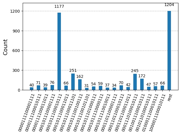
לאחר אופטימיזציה של המעגלים להרצת חומרה, אנחנו מוכנים להריץ אותם על חומרת היעד ולאסוף דגימות להערכת אנרגיית מצב היסוד. לאחר שימוש ב-primitive Sampler לדגום מחרוזות ביטים מכל מעגל, אנחנו משלבים את כל התוצאות למילון ספירה אחד ומתווים את 20 מחרוזות הביטים הנדגמות הנפוצות ביותר.
from qiskit.visualization import plot_histogram
from qiskit.primitives import StatevectorSampler

# Sample from the circuits
sampler = StatevectorSampler()
job = sampler.run(isa_circuits, shots=500)
from qiskit.primitives import BitArray

# Combine the shots from the individual Trotter circuits
bit_array = BitArray.concatenate_shots(
    [result.data.meas for result in job.result()]
)

plot_histogram(bit_array.get_counts(), number_to_keep=20)
שלב 4: עיבוד-המשך והחזרת התוצאה בפורמט הקלאסי הרצוי
כעת, אנחנו מריצים את אלגוריתם SQD באמצעות הפונקציה diagonalize_fermionic_hamiltonian. ראה את תיעוד ה-API להסברים על הארגומנטים לפונקציה זו.
from qiskit_addon_sqd.fermion import (
    SCIResult,
    diagonalize_fermionic_hamiltonian,
)

# List to capture intermediate results
result_history = []

def callback(results: list[SCIResult]):
    result_history.append(results)
    iteration = len(result_history)
    print(f"Iteration {iteration}")
    for i, result in enumerate(results):
        print(f"\tSubsample {i}")
        print(f"\t\tEnergy: {result.energy}")
        print(
            f"\t\tSubspace dimension: {np.prod(result.sci_state.amplitudes.shape)}"
        )

rng = np.random.default_rng(24)
result = diagonalize_fermionic_hamiltonian(
    h1e_momentum,
    h2e_momentum,
    bit_array,
    samples_per_batch=100,
    norb=norb,
    nelec=nelec,
    num_batches=3,
    max_iterations=5,
    symmetrize_spin=True,
    callback=callback,
    seed=rng,
)
Iteration 1
	Subsample 0
		Energy: -13.4222953188441
		Subspace dimension: 529
	Subsample 1
		Energy: -13.42237556285828
		Subspace dimension: 784
	Subsample 2
		Energy: -13.422045397387413
		Subspace dimension: 529
Iteration 2
	Subsample 0
		Energy: -13.422379583305478
		Subspace dimension: 900
	Subsample 1
		Energy: -13.422376197704326
		Subspace dimension: 841
	Subsample 2
		Energy: -13.422421162849295
		Subspace dimension: 1089
Iteration 3
	Subsample 0
		Energy: -13.422421164670345
		Subspace dimension: 1156
	Subsample 1
		Energy: -13.422421492737689
		Subspace dimension: 1156
	Subsample 2
		Energy: -13.422421205869572
		Subspace dimension: 1156
Iteration 4
	Subsample 0
		Energy: -13.422421494558726
		Subspace dimension: 1225
	Subsample 1
		Energy: -13.422421492737689
		Subspace dimension: 1156
	Subsample 2
		Energy: -13.422421492737689
		Subspace dimension: 1156
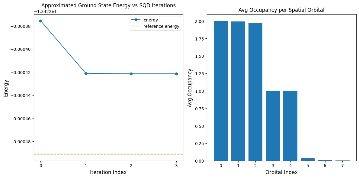
תא הקוד הבא משרטט את התוצאות. התרשים הראשון מציג את האנרגיה המחושבת כפונקציה של מספר איטרציות שחזור התצורה, והתרשים השני מציג את התפוסה הממוצעת של כל אורביטל מרחבי לאחר האיטרציה הסופית. מכיוון שמדובר בבעיה קטנה כל כך, האיטרציה הראשונה כבר מביאה אותנו קרוב מאוד לאנרגיה המדויקת (שים לב לסקלה של ציר ה-y).
import matplotlib.pyplot as plt

min_es = [
    min(result, key=lambda res: res.energy).energy
    for result in result_history
]
min_id, min_e = min(enumerate(min_es), key=lambda x: x[1])

# Data for energies plot
x1 = range(len(result_history))

# Data for avg spatial orbital occupancy
y2 = np.sum(result.orbital_occupancies, axis=0)
x2 = range(len(y2))

fig, axs = plt.subplots(1, 2, figsize=(12, 6))

# Plot energies
axs[0].plot(x1, min_es, label="energy", marker="o")
axs[0].set_xticks(x1)
axs[0].set_xticklabels(x1)
axs[0].axhline(
    y=reference_energy,
    color="#BF5700",
    linestyle="--",
    label="reference energy",
)
axs[0].set_title("Approximated Ground State Energy vs SQD Iterations")
axs[0].set_xlabel("Iteration Index", fontdict={"fontsize": 12})
axs[0].set_ylabel("Energy", fontdict={"fontsize": 12})
axs[0].legend()

# Plot orbital occupancy
axs[1].bar(x2, y2, width=0.8)
axs[1].set_xticks(x2)
axs[1].set_xticklabels(x2)
axs[1].set_title("Avg Occupancy per Spatial Orbital")
axs[1].set_xlabel("Orbital Index", fontdict={"fontsize": 12})
axs[1].set_ylabel("Avg Occupancy", fontdict={"fontsize": 12})

print(f"Reference energy: {reference_energy:.5f}")
print(f"SQD energy: {min_e:.5f}")
print(f"Absolute error: {abs(min_e - reference_energy):.5f}")
plt.tight_layout()
plt.show()
Reference energy: -13.42249
SQD energy: -13.42242
Absolute error: 0.00007
אמת את האנרגיה
האנרגיה המוחזרת על ידי SQD מובטחת להיות חסם עליון לאנרגיית מצב היסוד האמיתית. ניתן לאמת את הערך של האנרגיה מכיוון ש-SQD מחזיר גם את המקדמים של וקטור המצב המקרב את מצב היסוד. ניתן לחשב את האנרגיה מוקטור המצב באמצעות מטריצות הצפיפות המופחתות של חד-חלקיק ודו-חלקיק, כפי שמודגם בתא הקוד הבא.
rdm1 = result.sci_state.rdm(rank=1, spin_summed=True)
rdm2 = result.sci_state.rdm(rank=2, spin_summed=True)

energy = np.sum(h1e_momentum * rdm1) + 0.5 * np.sum(h2e_momentum * rdm2)

print(f"Recomputed energy: {energy:.5f}")
Recomputed energy: -13.42242
דוגמת חומרה בקנה מידה גדול
כעת, אנחנו מריצים דוגמה גדולה יותר על QPU אמיתי. עבור אנרגיית ההתייחסות, אנחנו משתמשים בתוצאות של חישוב DMRG שבוצע בנפרד.
from qiskit_ibm_runtime import SamplerV2 as Sampler
from qiskit_ibm_runtime import QiskitRuntimeService

# Model parameters
norb = 20
nelec = (norb // 2, norb // 2)
n_bath = norb - 1
hybridization = 1.0
hopping = 1.0
onsite = 10.0
chemical_potential = -0.5 * onsite

# Generate Hamiltonian and orbital rotation
h1e, h2e = siam_hamiltonian(
    norb=norb,
    hopping=hopping,
    onsite=onsite,
    hybridization=hybridization,
    chemical_potential=chemical_potential,
)
orbital_rotation = momentum_basis(norb)
h1e_momentum, h2e_momentum = rotated(h1e, h2e, orbital_rotation.T.conj())
impurity_index = n_bath // 2

# Set reference energy to DMRG value computed separately
reference_energy = -28.70659686

# Algorithm parameters
time_step = 0.2
krylov_dim = 8

# Construct circuits
qubits = QuantumRegister(2 * norb, name="q")
circuit = QuantumCircuit(qubits)
for instruction in prepare_initial_state(qubits, norb=norb, nocc=norb // 2):
    circuit.append(instruction)
circuit.measure_all()
circuits = [circuit.copy()]
one_body_evolution = scipy.linalg.expm(-1j * time_step * h1e_momentum)
for i in range(krylov_dim - 1):
    circuit.remove_final_measurements()
    for instruction in trotter_step(
        qubits,
        time_step,
        one_body_evolution,
        h2e_momentum,
        impurity_index,
        norb,
    ):
        circuit.append(instruction)
    circuit.measure_all()
    circuits.append(circuit.copy())

# Initialize hardware backend
service = QiskitRuntimeService()
backend = service.least_busy(
    operational=True, simulator=False, min_num_qubits=127
)
print(f"Using backend {backend.name}")

# Transpile to backend
pass_manager = generate_preset_pass_manager(
    optimization_level=3, backend=backend
)
isa_circuits = pass_manager.run(circuits)

# Sample from the circuits
sampler = Sampler(backend)
sampler.options.environment.job_tags = ["TUT_SKQD"]
job = sampler.run(isa_circuits, shots=500)

# Combine the shots from the individual Trotter circuits
bit_array = BitArray.concatenate_shots(
    [result.data.meas for result in job.result()]
)

# Run configuration recovery and diagonalization
result_history = []

def callback(results: list[SCIResult]):
    result_history.append(results)
    iteration = len(result_history)
    print(f"Iteration {iteration}")
    for i, result in enumerate(results):
        print(f"\tSubsample {i}")
        print(f"\t\tEnergy: {result.energy}")
        print(
            f"\t\tSubspace dimension: {np.prod(result.sci_state.amplitudes.shape)}"
        )

rng = np.random.default_rng(24)
result = diagonalize_fermionic_hamiltonian(
    h1e_momentum,
    h2e_momentum,
    bit_array,
    samples_per_batch=100,
    norb=norb,
    nelec=nelec,
    num_batches=3,
    max_iterations=5,
    symmetrize_spin=True,
    callback=callback,
    seed=rng,
)

# Plot results
min_es = [
    min(result, key=lambda res: res.energy).energy
    for result in result_history
]
min_id, min_e = min(enumerate(min_es), key=lambda x: x[1])
x1 = range(len(result_history))
y2 = np.sum(result.orbital_occupancies, axis=0)
x2 = range(len(y2))
fig, axs = plt.subplots(1, 2, figsize=(12, 6))
axs[0].plot(x1, min_es, label="energy", marker="o")
axs[0].set_xticks(x1)
axs[0].set_xticklabels(x1)
axs[0].axhline(
    y=reference_energy,
    color="#BF5700",
    linestyle="--",
    label="reference energy",
)
axs[0].set_title("Approximated Ground State Energy vs SQD Iterations")
axs[0].set_xlabel("Iteration Index", fontdict={"fontsize": 12})
axs[0].set_ylabel("Energy", fontdict={"fontsize": 12})
axs[0].legend()
axs[1].bar(x2, y2, width=0.8)
axs[1].set_xticks(x2)
axs[1].set_xticklabels(x2)
axs[1].set_title("Avg Occupancy per Spatial Orbital")
axs[1].set_xlabel("Orbital Index", fontdict={"fontsize": 12})
axs[1].set_ylabel("Avg Occupancy", fontdict={"fontsize": 12})
print(f"Reference energy: {reference_energy:.5f}")
print(f"SQD energy: {min_e:.5f}")
print(f"Absolute error: {abs(min_e - reference_energy):.5f}")
plt.tight_layout()
plt.show()
Using backend ibm_boston
Iteration 1
	Subsample 0
		Energy: -28.63965951544449
		Subspace dimension: 9801
	Subsample 1
		Energy: -28.625588929202006
		Subspace dimension: 9409
	Subsample 2
		Energy: -28.647371834135498
		Subspace dimension: 8281
Iteration 2
	Subsample 0
		Energy: -28.67213260849567
		Subspace dimension: 29584
	Subsample 1
		Energy: -28.670340686158816
		Subspace dimension: 27225
	Subsample 2
		Energy: -28.669976379525988
		Subspace dimension: 31329
Iteration 3
	Subsample 0
		Energy: -28.68622875601382
		Subspace dimension: 36100
	Subsample 1
		Energy: -28.698569623143126
		Subspace dimension: 34225
	Subsample 2
		Energy: -28.694848533971882
		Subspace dimension: 33856
Iteration 4
	Subsample 0
		Energy: -28.69883392844593
		Subspace dimension: 42025
	Subsample 1
		Energy: -28.701289495200996
		Subspace dimension: 38025
	Subsample 2
		Energy: -28.699319594978245
		Subspace dimension: 45369
Iteration 5
	Subsample 0
		Energy: -28.701936886834154
		Subspace dimension: 51076
	Subsample 1
		Energy: -28.702468711812013
		Subspace dimension: 53824
	Subsample 2
		Energy: -28.702298147575938
		Subspace dimension: 52900
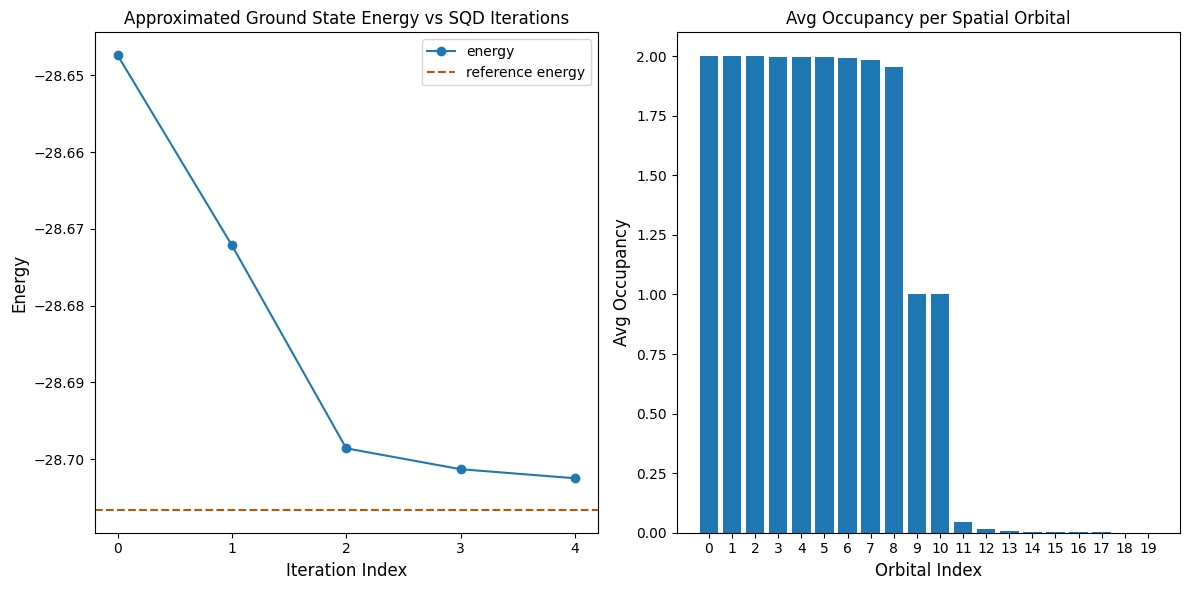
Reference energy: -28.70660
SQD energy: -28.70247
Absolute error: 0.00413
הצעדים הבאים
אם מצאת עבודה זו מעניינת, ייתכן שתתעניין בחומר הבא:
- ליכסון קוונטי מבוסס-דגימה של המילטוניאן כימי - מדריך קשור המשתמש ב-ansatz וריאציוני היוריסטי במקום מעגלי Trotter
- ליכסון קוונטי Krylov של המילטוניאני סריג - מדריך על שיטת KQD
- תיעוד ה-API של SQD addon - עיון בפונקציה
diagonalize_fermionic_hamiltonian - Quantum-Centric Algorithm for Sample-Based Krylov Diagonalization - המאמר עליו מבוסס מדריך זה