מבחן ביצועים להטלת אופרטור פאולי

פעולת מחרוזת פאולי על מצב בסיס חישובי

הפעולה של מחרוזת פאולי על מצב בסיס חישובי היא טריוויאלית למדי, והתוצאה היא עצמה מצב בסיס חישובי יחיד. זו תוצאה ישירה של מבנה מטריצות פאולי, שיש בהן רק איבר שונה מאפס אחד בכל שורה. לכן הפעולה שלהן על qubit היא:

---

$$\sigma_x |0 \rangle = |1 \rangle$$ $$\sigma_x |1 \rangle = |0 \rangle$$

---

$$\sigma_y |0 \rangle = i|1 \rangle$$ $$\sigma_y |1 \rangle = -i|0 \rangle$$

---

$$\sigma_z |0 \rangle = |0 \rangle$$ $$\sigma_z |1 \rangle = -|1 \rangle$$

---

$$I |0 \rangle = |0 \rangle$$ $$I |1 \rangle = |1 \rangle$$

---

כל ביט במחרוזת הביטים שמסמנת את הבסיס החישובי יסומן ב-$x \in \{0, 1 \}$. כדי לשמור על מימוש קל ככל האפשר, נייצג את מחרוזות הביטים באמצעות משתנים מסוג bool: $0\rightarrow \textrm{False}$ ו-$1\rightarrow \textrm{True}$.

כדי לייצג את הפעולה של כל אופרטור פאולי על מצב בסיס חישובי, נקצה לו שלושה משתנים: diag, sign, imag.

• diag מציין אם האופרטור אלכסוני:

  • $\textrm{diag}(I) = \textrm{True}$

  • $\textrm{diag}(\sigma_x) = \textrm{False}$

  • $\textrm{diag}(\sigma_y) = \textrm{False}$

  • $\textrm{diag}(\sigma_z) = \textrm{True}$

• sign מציין אם יש שינוי סימן באיבר המטריצה שמחובר ל-0 או ל-1:

  • $\textrm{sign}(I) = \textrm{False}$

  • $\textrm{sign}(\sigma_x) = \textrm{False}$

  • $\textrm{sign}(\sigma_y) = \textrm{True}$

  • $\textrm{sign}(\sigma_z) = \textrm{True}$

• imag מציין אם יש רכיב מרוכב באיבר המטריצה:

  • $\textrm{imag}(I) = \textrm{False}$

  • $\textrm{imag}(\sigma_x) = \textrm{False}$

  • $\textrm{imag}(\sigma_y) = \textrm{True}$

  • $\textrm{imag}(\sigma_z) = \textrm{False}$

אנחנו מסמנים אופרטור פאולי כלשהו ב-$\sigma \in \{ I, \sigma_x, \sigma_y \sigma_z\}$. את הפעולה של אופרטור פאולי על מצב בסיס חישובי אפשר לייצג בפעולה הלוגית:

$$\sigma |x \rangle = |x == \textrm{diag}(\sigma) \rangle (-1)^{x\textrm{ and sign}(\sigma)} (i)^{\textrm{imag}(\sigma)}.$$

אותו דבר מוכלל בקלות למספר שרירותי של qubits. בואו נבדוק שזה עובד:

# Added by doQumentation — installs the packages this notebook needs if they are missing
import importlib.util

_needed = {"matplotlib": "matplotlib", "numpy": "numpy", "qiskit": "qiskit", "qiskit_addon_sqd": "qiskit-addon-sqd"}
_missing = [pip for module, pip in _needed.items()
            if importlib.util.find_spec(module) is None]
# One at a time, so a package that fails to install does not block the others
for _pip in _missing:
    %pip install -q {_pip}
if not _missing:
    print("\u2713 All required packages are installed")

def connected_element_and_amplitude_bool(
    x: bool, diag: bool, sign: bool, imag: bool
) -> tuple[bool, complex]:
    """
    Finds the connected element to computational basis state |x> under
    the action of the Pauli operator represented by (diag, sign, imag).

    Args:
        x: Value of the bit, either True or False.
        diag: Whether the Pauli operator is diagonal (I, Z)
        sigma: Whether the Pauli operator's rows differ in sign (Y, Z)
        imag: Whether the Pauli operator is purely imaginary (Y)

    Returns:
        A length-2 tuple:
            - The connected element to x, either False or True
            - The matrix element
    """
    return x == diag, (-1) ** (x and sign) * (1j) ** (imag)

sigma_indices = [0, 1, 2, 3]
sigma_string = ["I", "SX", "SZ", "SY"]
sigma_diag = [True, False, True, False]
sigma_sign = [False, False, True, True]
sigma_imag = [False, False, False, True]
qubit_values = [False, True]

for xi in sigma_indices:
    print("-------------------")
    print(sigma_string[xi])
    for x in qubit_values:
        x_p, matrix_element = connected_element_and_amplitude_bool(
            x, sigma_diag[xi], sigma_sign[xi], sigma_imag[xi]
        )
        print(
            "|"
            + str(x)
            + "> -->  |"
            + str(x_p)
            + ">    ME:"
            + str(matrix_element)
        )

-------------------
I
|False> -->  |False>    ME:(1+0j)
|True> -->  |True>    ME:(1+0j)
-------------------
SX
|False> -->  |True>    ME:(1+0j)
|True> -->  |False>    ME:(1+0j)
-------------------
SZ
|False> -->  |False>    ME:(1+0j)
|True> -->  |True>    ME:(-1+0j)
-------------------
SY
|False> -->  |True>    ME:1j
|True> -->  |False>    ME:(-0-1j)

אנחנו יוצרים מספר גדול של מחרוזות ביטים (50 מיליון) עבור מערכת של 40 qubits:

import numpy as np
from qiskit_addon_sqd.qubit import sort_and_remove_duplicates

rand_seed = 22
np.random.seed(rand_seed)

# Generate some random bitstrings for testing

def random_bitstrings(n_samples, n_qubits):
    return (
        np.round(np.random.rand(n_samples, n_qubits))
        .astype("int")
        .astype("bool")
    )

n_qubits = 40
bts_matrix = random_bitstrings(50_000_000, n_qubits)

# We need to sort the bitstrings and only keep the unique ones
# NOTE: It is essential for the projection code to have the bitstrings sorted!
bts_matrix = sort_and_remove_duplicates(bts_matrix).astype("bool")

# Final subspace dimension after getting rid of duplicated bitstrings
d = bts_matrix.shape[0]

print("Total number of unique bitstrings: " + str(d))

Total number of unique bitstrings: 49998839

מבחן ביצועים לפונקציות הטלת פאולי ב-SQD

מחרוזת פאולי הנבחנת היא $\sigma_z \otimes ... \otimes \sigma_z$.

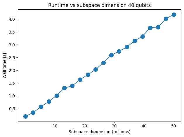
מימדי תת-מרחב שונים נבחנים על ידי חיתוך מטריצת מחרוזות הביטים. אנחנו מודדים את זמן ההטלה לתת-המרחב עבור גדלי תת-מרחב שונים.

import time

from qiskit.quantum_info import Pauli
from qiskit_addon_sqd.qubit import matrix_elements_from_pauli

pauli = Pauli("Z" * n_qubits)

# Different subspace sizes to test
d_list = np.linspace(d / 1000, d, 20).astype("int")

# To store the walltime
time_array = np.zeros(20)

for i in range(20):
    int_bts_matrix = bts_matrix[: d_list[i], :]
    time_1 = time.time()
    _ = matrix_elements_from_pauli(int_bts_matrix, pauli)
    time_array[i] = time.time() - time_1
    print(f"Iteration {i} took {round(time_array[i], 6)}s")

Iteration 0 took 0.201246s
Iteration 1 took 0.348222s
Iteration 2 took 0.576333s
Iteration 3 took 0.78356s
Iteration 4 took 1.016162s
Iteration 5 took 1.305325s
Iteration 6 took 1.392751s
Iteration 7 took 1.632433s
Iteration 8 took 1.826521s
Iteration 9 took 2.02903s
Iteration 10 took 2.297458s
Iteration 11 took 2.588042s
Iteration 12 took 2.738746s
Iteration 13 took 2.906144s
Iteration 14 took 3.148833s
Iteration 15 took 3.323253s
Iteration 16 took 3.664171s
Iteration 17 took 3.680663s
Iteration 18 took 4.008313s
Iteration 19 took 4.173532s

import matplotlib.pyplot as plt

# Data for energies plot
x1 = d_list
y1 = time_array

# Plot energies
plt.title("Runtime vs subspace dimension 40 qubits")
plt.xlabel("Subspace dimension (millions)")
plt.ylabel("Wall time [s]")
plt.xticks([1e7, 2e7, 3e7, 4e7, 5e7], [str(i) for i in [10, 20, 30, 40, 50]])
plt.plot(x1, y1, marker=".", markersize=20)
plt.tight_layout()
plt.show()

עכשיו נעשה את אותו דבר עבור 60 qubits:

n_qubits = 60
bts_matrix = random_bitstrings(50_000_000, n_qubits)

# We need to sort the bitstrings and just keep the unique ones
bts_matrix = sort_and_remove_duplicates(bts_matrix).astype("bool")

# Final subspace dimension after getting rid of duplicated bitstrings
d = bts_matrix.shape[0]

print("Total number of unique bitstrings: " + str(d))

Total number of unique bitstrings: 50000000

pauli = Pauli("Z" * n_qubits)

# Different subspace sizes to test
d_list = np.linspace(d / 1000, d, 20).astype("int")

# It is better to do this once
row_array = np.arange(d)

# To store the walltime
time_array = np.zeros(20)

for i in range(20):
    int_bts_matrix = bts_matrix[: d_list[i], :]
    int_row_array = row_array[: d_list[i]]
    time_1 = time.time()
    _ = matrix_elements_from_pauli(int_bts_matrix, pauli)
    time_array[i] = time.time() - time_1
    print(f"Iteration {i} took {round(time_array[i], 6)}s")

Iteration 0 took 0.236567s
Iteration 1 took 0.424116s
Iteration 2 took 0.673399s
Iteration 3 took 0.905164s
Iteration 4 took 1.168936s
Iteration 5 took 1.454204s
Iteration 6 took 1.74778s
Iteration 7 took 1.920795s
Iteration 8 took 2.259994s
Iteration 9 took 2.550674s
Iteration 10 took 2.681287s
Iteration 11 took 3.04411s
Iteration 12 took 3.293262s
Iteration 13 took 3.471247s
Iteration 14 took 3.726639s
Iteration 15 took 4.072854s
Iteration 16 took 4.221037s
Iteration 17 took 4.498535s
Iteration 18 took 4.741108s
Iteration 19 took 5.159038s

# Data for energies plot
x1 = d_list
y1 = time_array

fig, axs = plt.subplots(1, 1, figsize=(6, 6))

# Plot energies
axs.plot(x1, y1, marker=".", markersize=20)
axs.set_title("Runtime vs subspace dimension 60 qubits")
axs.set_xlabel("Subspace dimension (millions)")
plt.xticks([1e7, 2e7, 3e7, 4e7, 5e7], [str(i) for i in [10, 20, 30, 40, 50]])
axs.set_ylabel("Wall time [s]")

plt.tight_layout()
plt.show()