הגבלת מימד תת-המרחב

במדריך הזה נראה את ההשפעה של מימד תת-המרחב בטכניקת שחזור התצורות העקבי-עצמית.

A priori, אנחנו לא יודעים מהו מימד תת-המרחב הנכון כדי להגיע לרמת דיוק יעד. עם זאת, אנחנו כן יודעים שהגדלת מימד תת-המרחב מגדילה את דיוק השיטה. לכן אפשר לחקור את דיוק התחזיות כפונקציה של מימד תת-המרחב. הגדירו את המולקולה ואת תכונותיה.

# Added by doQumentation — installs the packages this notebook needs if they are missing
import importlib.util

_needed = {"matplotlib": "matplotlib", "numpy": "numpy", "pyscf": "pyscf", "qiskit_addon_sqd": "qiskit-addon-sqd"}
_missing = [pip for module, pip in _needed.items()
            if importlib.util.find_spec(module) is None]
# One at a time, so a package that fails to install does not block the others
for _pip in _missing:
    %pip install -q {_pip}
if not _missing:
    print("\u2713 All required packages are installed")

import warnings

import pyscf
import pyscf.cc
import pyscf.mcscf

warnings.filterwarnings("ignore")

# Specify molecule properties
open_shell = False
spin_sq = 0

# Build N2 molecule
mol = pyscf.gto.Mole()
mol.build(
    atom=[["N", (0, 0, 0)], ["N", (1.0, 0, 0)]],
    basis="6-31g",
    symmetry="Dooh",
)

# Define active space
n_frozen = 2
active_space = range(n_frozen, mol.nao_nr())

# Get molecular integrals
scf = pyscf.scf.RHF(mol).run()
num_orbitals = len(active_space)
n_electrons = int(sum(scf.mo_occ[active_space]))
num_elec_a = (n_electrons + mol.spin) // 2
num_elec_b = (n_electrons - mol.spin) // 2
cas = pyscf.mcscf.CASCI(scf, num_orbitals, (num_elec_a, num_elec_b))
mo = cas.sort_mo(active_space, base=0)
hcore, nuclear_repulsion_energy = cas.get_h1cas(mo)
eri = pyscf.ao2mo.restore(1, cas.get_h2cas(mo), num_orbitals)

# Compute exact energy
exact_energy = cas.run().e_tot

converged SCF energy = -108.835236570775
CASCI E = -109.046671778080  E(CI) = -32.8155692383188  S^2 = 0.0000000

צרו מחרוזות ביטים אקראיות שישמשו כתחליף לדגימות QPU.

import numpy as np
from qiskit_addon_sqd.counts import generate_bit_array_uniform

# Create a seed to control randomness throughout this workflow
rng = np.random.default_rng(24)

# Generate random samples
bit_array = generate_bit_array_uniform(
    10_000, num_orbitals * 2, rand_seed=rng
)

הריצו את SQD עם גדלי אצווה הולכים וגדלים.

from qiskit_addon_sqd.fermion import diagonalize_fermionic_hamiltonian

list_samples_per_batch = [50, 200, 400, 600]

# SQD options
max_iterations = 5

# Eigenstate solver options
num_batches = 10
max_davidson_cycles = 200

energies = []
subspace_dimensions = []

for samples_per_batch in list_samples_per_batch:
    result = diagonalize_fermionic_hamiltonian(
        hcore,
        eri,
        bit_array,
        samples_per_batch=samples_per_batch,
        norb=num_orbitals,
        nelec=(num_elec_a, num_elec_b),
        num_batches=num_batches,
        max_iterations=max_iterations,
        symmetrize_spin=True,
        seed=rng,
    )
    energies.append(result.energy)
    subspace_dimensions.append(np.prod(result.sci_state.amplitudes.shape))

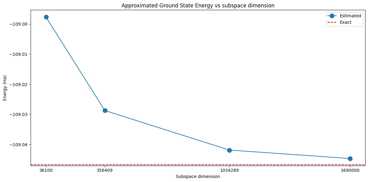
הגרף הזה מראה שהגדלת מימד תת-המרחב מובילה לתוצאות מדויקות יותר.

import matplotlib.pyplot as plt

# Data for energies plot
x1 = subspace_dimensions
y1 = np.array(energies) + nuclear_repulsion_energy

fig, axs = plt.subplots(1, 1, figsize=(12, 6))

# Plot energies
axs.plot(x1, y1, marker=".", markersize=20, label="Estimated")
axs.set_xticks(x1)
axs.set_xticklabels(x1)
axs.axhline(y=exact_energy, color="red", linestyle="--", label="Exact")
axs.set_title("Approximated Ground State Energy vs subspace dimension")
axs.set_xlabel("Subspace dimension")
axs.set_ylabel("Energy (Ha)")
axs.legend()

plt.tight_layout()
plt.show()

הגדרת חסם מפורש באמצעות max_dim

בסריקה שלמעלה, מימד תת-המרחב נשלט רק בעקיפין. samples_per_batch קובע כמה מחרוזות ביטים נשלפות לכל אצווה, אבל המימד של תת-המרחב שמתקבל נקבע לפי מספר מחרוזות הספין-אלפא והספין-בטא השונות שמחרוזות הביטים האלה מכילות, ומאגר התצורות הזמין לדגימה משנית גדל מאיטרציית שחזור תצורות אחת לבאה אחריה. לכן מימדי תת-המרחב בציר האופקי שלמעלה הם מספרים לא סדירים שלא בחרנו.

הארגומנט max_dim של diagonalize_fermionic_hamiltonian מגביל את המימד ישירות. הוא מגביל את מספר מחרוזות ה-CI שנשמרות בכל מגזר ספין, ומכיוון שתת-המרחב נפרש על ידי המכפלה הקרטזית של שני המגזרים, המימד שלו הוא מכפלת המימדים של שני המגזרים:

• max_dim=d מגביל את שני המגזרים ל-d מחרוזות, כך שמימד תת-המרחב הוא לכל היותר d ** 2.

• max_dim=(d_a, d_b) מגביל את מגזרי הספין-אלפא והספין-בטא בנפרד, כך שמימד תת-המרחב הוא לכל היותר d_a * d_b. כאשר symmetrize_spin=True, שני הגבולות חייבים להיות שווים.

• max_dim=None, ברירת המחדל, לא מטיל שום הגבלה.

כשאצווה מכילה יותר מחרוזות ממה שההגבלה מאפשרת, החשובות פחות נזרקות: קודם נשמרות המחרוזות שהועברו דרך include_configurations, אחריהן המחרוזות שהועברו מהאיטרציה הקודמת (ראו carryover_threshold), והמקומות שנשארים מתמלאים במחרוזות שנדגמו, לפי סדר יורד של תדירות הדגימה שלהן.

מכיוון ש-max_dim חוסם את גודל ההאלכסון הגדול ביותר שפותר הערכים העצמיים יתבקש לבצע, זו דרך נוחה להחזיק את הפותר בתוך תקציב של זמן ריצה וזיכרון: בחרו samples_per_batch בנדיבות, ותנו ל-max_dim להחליט עד כמה תת-המרחב יכול לגדול.

להלן נחזור על המחקר, והפעם נשאיר את samples_per_batch קבוע ונגדיל את max_dim.

list_max_dim = [100, 200, 400, 800]

# Use a generous number of samples per batch, so that max_dim is what limits
# the dimension of the subspace
samples_per_batch = 600

energies_max_dim = []
subspace_dimensions_max_dim = []

for max_dim in list_max_dim:
    result = diagonalize_fermionic_hamiltonian(
        hcore,
        eri,
        bit_array,
        samples_per_batch=samples_per_batch,
        norb=num_orbitals,
        nelec=(num_elec_a, num_elec_b),
        num_batches=num_batches,
        max_iterations=max_iterations,
        symmetrize_spin=True,
        max_dim=max_dim,
        seed=rng,
    )
    energies_max_dim.append(result.energy)
    subspace_dimensions_max_dim.append(
        int(np.prod(result.sci_state.amplitudes.shape))
    )

print(f"max_dim:            {list_max_dim}")
print(f"subspace dimension: {subspace_dimensions_max_dim}")

max_dim:            [100, 200, 400, 800]
subspace dimension: [10000, 40000, 160000, 640000]

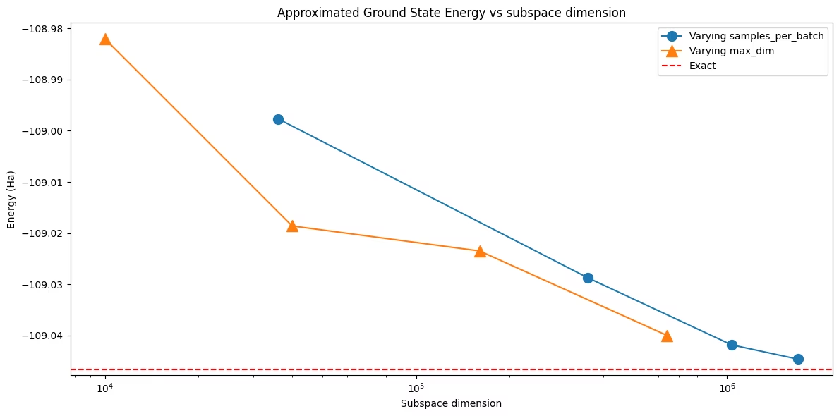
מימד תת-המרחב הוא עכשיו בדיוק max_dim ** 2 בכל הרצה: הוא נבחר ולא התגלה. הצגת שתי הסריקות יחד מראה שהדיוק נקבע לפי מימד תת-המרחב עצמו, בלי קשר לארגומנט ששימש להגיע אליו. עם זאת, שני העקומים לא חייבים להתלכד בדיוק. הרצות max_dim שולפות 600 מחרוזות ביטים לכל אצווה ואז שומרות את המחרוזות שנדגמו בתדירות הגבוהה ביותר, ולכן במימד נתון הן יכולות לשמור קבוצת תצורות טובה יותר מהרצה שהגיעה לאותו מימד בכך שדגמה מלכתחילה פחות מחרוזות ביטים.

fig, axs = plt.subplots(1, 1, figsize=(12, 6))

axs.plot(
    subspace_dimensions,
    np.array(energies) + nuclear_repulsion_energy,
    marker=".",
    markersize=20,
    label="Varying samples_per_batch",
)
axs.plot(
    subspace_dimensions_max_dim,
    np.array(energies_max_dim) + nuclear_repulsion_energy,
    marker="^",
    markersize=12,
    label="Varying max_dim",
)
axs.axhline(y=exact_energy, color="red", linestyle="--", label="Exact")
axs.set_xscale("log")
axs.ticklabel_format(axis="y", useOffset=False)
axs.set_title("Approximated Ground State Energy vs subspace dimension")
axs.set_xlabel("Subspace dimension")
axs.set_ylabel("Energy (Ha)")
axs.legend()

plt.tight_layout()
plt.show()