קידוד נתונים

מבוא וסימונים

כדי להשתמש באלגוריתם קוונטי, יש להכניס נתונים קלאסיים לתוך Circuit קוונטי. לכך מתייחסים בדרך כלל כקידוד נתונים, אך גם כטעינת נתונים. נזכיר משיעורים קודמים את מושג המיפוי של תכונות — מיפוי של תכונות נתונים ממרחב אחד למשנהו. העברה של נתונים קלאסיים למחשב קוונטי היא סוג של מיפוי, שאפשר לקרוא לו מיפוי תכונות. בפועל, מיפויי התכונות המובנים ב-Qiskit (כמו z_Feature Map ו-ZZ Feature Map) יכללו בדרך כלל שכבות סיבוב ושכבות שזירה המרחיבות את המצב לממדים רבים במרחב הילברט. תהליך הקידוד הזה הוא חלק קריטי באלגוריתמי למידת מכונה קוונטיים ומשפיע ישירות על היכולות החישוביות שלהם.

חלק מטכניקות הקידוד שלהלן ניתנות לסימולציה קלאסית יעילה; קל במיוחד לראות זאת בשיטות קידוד המניבות מצבי מכפלה (כלומר, אינן שוזרות Qubitים). וכדאי לזכור שסביר שהיתרון הקוונטי יימצא דווקא כאשר המורכבות הקוונטית של מערך הנתונים מתאימה היטב לשיטת הקידוד. לכן סביר מאוד שבסופו של דבר תכתוב Circuit קידוד משלך. כאן אנו מציגים מגוון רחב של אסטרטגיות קידוד אפשריות כדי שתוכל להשוות ביניהן ולראות מה אפשרי. אפשר לומר כמה דברים כלליים על יעילות טכניקות הקידוד. לדוגמה, efficient_su2 (ראה להלן) עם סכמת שזירה מלאה סביר הרבה יותר שיתפוס תכונות קוונטיות של נתונים מאשר שיטות המניבות מצבי מכפלה (כמו z_feature_map). אך אין זה אומר ש-efficient_su2 מספיק, או מתאים מספיק למערך הנתונים שלך, כדי להניב האצה קוונטית. הדבר מצריך בחינה מדוקדקת של מבנה הנתונים שמנסים למדל או לסווג. יש גם פשרה עם עומק ה-Circuit, שכן מיפויי תכונות רבים שמשזרים את כל ה-Qubitים ב-Circuit מניבים Circuitים עמוקים מאוד, עמוקים מדי לקבלת תוצאות שמישות על המחשבים הקוונטיים של היום.

סימונים

מערך נתונים הוא קבוצה של $M$ וקטורי נתונים: $\text{X} = \{\vec{x}^{(j)}\,|\,j\in [M]\}$, כאשר כל וקטור הוא בעל $N$ ממדים, כלומר $\vec{x}^{(j)}=(\vec{x}^{(j)}_1,\ldots,\vec{x}^{(j)}_N)\in\mathbb{R}^N$. ניתן להרחיב זאת לתכונות נתונים מרוכבות. בשיעור זה, נשתמש לעיתים בסימונים אלה עבור הקבוצה המלאה $(\text{X})$ ועבור אלמנטים ספציפיים שלה כמו $\vec{x}^{(j)}$. אך בעיקר נתייחס לטעינה של וקטור יחיד ממערך הנתונים שלנו בכל פעם, ולרוב נתייחס פשוט לוקטור יחיד בן $N$ תכונות בתור $\vec{x}$.

בנוסף, נהוג להשתמש בסמל $\Phi(\vec{x})$ כדי לציין את מיפוי התכונות $\Phi$ של וקטור הנתונים $\vec{x}$. בתכנות קוונטי ספציפית, נהוג לציין מיפויים בעזרת $U(\vec{x})$, סימון המדגיש את האופי האוניטרי של פעולות אלו. ניתן להשתמש באותו סמל לשניהם כיאות; שניהם הם מיפויי תכונות. לאורך קורס זה, אנו נוטים להשתמש ב:

• $\Phi(\vec{x})$ כאשר אנו דנים במיפויי תכונות בלמידת מכונה באופן כללי, ו
• $U(\vec{x})$ כאשר אנו דנים במימושי Circuit של מיפויי תכונות.

נורמליזציה ואובדן מידע

בלמידת מכונה קלאסית, תכונות של נתוני אימון מנורמלות או מוצרות לרוב מחדש, מה שמשפר לעיתים קרובות את ביצועי המודל. דרך נפוצה אחת לעשות זאת היא נורמליזציית מינימום-מקסימום או סטנדרטיזציה. בנורמליזציית מינימום-מקסימום, עמודות תכונות של מטריצת הנתונים $\text{X}$ (נאמר, תכונה $k$) מנורמלות:

$$x^{'(i)}_k = \frac{x^{(i)}_k - \text{min}\{x^{(j)}_k\,|\,\vec{x}^{(j)}\in [\text{X}]\}}{\text{max}\{x^{(j)}_k\,|\,\vec{x}^{(j)}\in [\text{X}]\}-\text{min}\{x^{(j)}_k\,|\,\vec{x}^{(j)}\in [\text{X}]\}}$$

כאשר מינימום ומקסימום מתייחסים למינימום ולמקסימום של תכונה $k$ על פני $M$ וקטורי הנתונים במערך $\text{X}$. כל ערכי התכונות נופלים אז בקטע היחידה: $x^{'(i)}_k \in [0,1]$ לכל $i\in [M]$, $k\in[N]$.

נורמליזציה היא גם מושג יסודי במכניקת הקוונטים ובתכנות קוונטי, אך היא שונה במקצת מנורמליזציית מינימום-מקסימום. נורמליזציה במכניקת הקוונטים מחייבת שהאורך (בהקשר של תכנות קוונטי, הנורמה-2) של וקטור המצב $|\psi\rangle$ שווה לאחד: $\|\psi\|=\sqrt{\langle\psi|\psi\rangle} = 1$, המבטיח שסכום ההסתברויות של המדידה שווה ל-1. המצב מנורמל על ידי חלוקה בנורמה-2; כלומר, על ידי סיכול מחדש

$$|\psi\rangle\rightarrow\|\psi\|^{-1}|\psi\rangle$$

בתכנות קוונטי ובמכניקת הקוונטים, זוהי לא נורמליזציה שאנשים מטילים על הנתונים, אלא תכונה יסודית של מצבים קוונטיים. בהתאם לסכמת הקידוד שלך, אילוץ זה עשוי להשפיע על האופן שבו הנתונים שלך מוצרים מחדש. לדוגמה, בקידוד אמפליטודה (ראה להלן), וקטור הנתונים מנורמל $\vert\vec{x}^{(j)}\vert = 1$ כנדרש על ידי מכניקת הקוונטים, וזה משפיע על המידות של הנתונים המקודדים. בקידוד פאזה, מומלץ לסכם מחדש את ערכי התכונות כ-$\vec{x}^{(j)}_i \in (0,2\pi]$ כדי שלא יהיה אובדן מידע עקב אפקט המודולו-$2\pi$ של הקידוד לזווית פאזה של Qubit[1,2].

שיטות קידוד

בכמה הסעיפים הבאים, נתייחס למערך נתונים קלאסי לדוגמה קטן $\text{X}_\text{ex}$ המורכב מ-$M=5$ וקטורי נתונים, כל אחד בעל $N=3$ תכונות:

$$\text{X}_{\text{ex}}=\{(4,8,5),(9,8,6),(2,9,2),(5,7,0),(3,7,5)\}$$

בסימונים שהוצגו לעיל, נוכל לומר שהתכונה ה-$1^\text{st}$ של וקטור הנתונים ה-$4^\text{th}$ בקבוצה שלנו $\text{X}_{\text{ex}}$ היא $\vec{x}^{(4)}_1 = 5$, לדוגמה.

קידוד בסיס

קידוד בסיס מקודד מחרוזת $P$-ביטים קלאסית למצב בסיס חישובי של מערכת $P$-Qubit. נניח לדוגמה $\vec{x}^{(1)}_3 = 5 = 0(2^3)+1(2^2)+0(2^1)+1(2^0)$. ניתן לייצג זאת כמחרוזת $4$-ביטים $(0101)$, ועל ידי מערכת $4$-Qubit כמצב קוונטי $|0101\rangle$. באופן כללי יותר, עבור מחרוזת $P$-ביטים: $\vec{x}^{(j)}_k = (b_1, b_2, ... , b_P)$, מצב ה-$P$-Qubit המתאים הוא $|x^{(j)}_k\rangle = | b_1, b_2, ... , b_P \rangle$ כאשר $b_n \in \{0,1\}$ עבור $n = 1 , \dots , P$. שים לב שזה עבור תכונה בודדת.

קידוד בסיס בתכנות קוונטי מייצג כל סיבית קלאסית כ-Qubit נפרד, ממפה את הייצוג הבינארי של הנתונים ישירות למצבים קוונטיים בבסיס החישובי. כאשר צריך לקודד תכונות מרובות, כל תכונה מומרת תחילה לצורתה הבינארית ולאחר מכן מוקצית לקבוצה נפרדת של Qubitים — קבוצה אחת לכל תכונה — כאשר כל Qubit משקף סיבית בייצוג הבינארי של אותה תכונה.

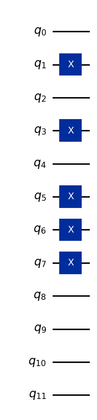
כדוגמה, בוא נקודד את הוקטור (5, 7, 0).

נניח שכל התכונות מאוחסנות בארבעה ביטים (יותר ממה שצריך, אבל מספיק לייצוג כל מספר שלם בעל ספרה אחת בבסיס 10):

5 → binary 0101

7 → binary 0111

0 → binary 0000

מחרוזות ביטים אלה מוקצות לשלוש קבוצות של ארבעה Qubitים כל אחת, ולכן מצב הבסיס הכולל של 12 Qubit הוא:

$$∣0101 0111 0000⟩$$

כאן, ארבעת ה-Qubitים הראשונים מייצגים את התכונה הראשונה, ארבעת ה-Qubitים הבאים את התכונה השנייה, וארבעת ה-Qubitים האחרונים את התכונה השלישית. הקוד להלן ממיר את וקטור הנתונים (5,7,0) למצב קוונטי, ומוכלל לעשות זאת עבור תכונות אחרות בעלות ספרה אחת.

# Added by doQumentation — required packages for this notebook
!pip install -q matplotlib numpy qiskit

from qiskit import QuantumCircuit

# Data point to encode
x = 5  # binary: 0101
y = 7  # binary: 0111
z = 0  # binary: 0000

# Convert each to 4-bit binary list
x_bits = [int(b) for b in format(x, "04b")]  # [0,1,0,1]
y_bits = [int(b) for b in format(y, "04b")]  # [0,1,1,1]
z_bits = [int(b) for b in format(z, "04b")]  # [0,0,0,0]

# Combine all bits
all_bits = x_bits + y_bits + z_bits  # [0,1,0,1,0,1,1,1,0,0,0,0]

# Initialize a 12-qubit quantum circuit
qc = QuantumCircuit(12)

# Apply x-gates where the bit is 1
for idx, bit in enumerate(all_bits):
    if bit == 1:
        qc.x(idx)

qc.draw("mpl")

בדוק את הבנתך

קרא את השאלה למטה, חשוב על תשובתך, ולאחר מכן לחץ על המשולש לחשיפת הפתרון.

כתוב קוד לקידוד הוקטור הראשון במערך הנתונים לדוגמה שלנו $\text{X}_{\text{ex}}$:

$\vec{x}^{(1)}=(4,8,5)$

באמצעות קידוד בסיס.

תשובה:

import math
from qiskit import QuantumCircuit

# Data point to encode
x = 4  # binary: 0100
y = 8  # binary: 1000
z = 5  # binary: 0101

# Convert each to 4-bit binary list
x_bits = [int(b) for b in format(x, '04b')]  # [0,1,0,0]
y_bits = [int(b) for b in format(y, '04b')]  # [1,0,0,0]
z_bits = [int(b) for b in format(z, '04b')]  # [0,1,0,1]

# Combine all bits
all_bits = x_bits + y_bits + z_bits  # [0,1,0,0,1,0,0,0,0,1,0,1]

# Initialize a 12-qubit quantum circuit
qc = QuantumCircuit(12)

# Apply x-gates where the bit is 1
for idx, bit in enumerate(all_bits):
    if bit == 1:
        qc.x(idx)

qc.draw('mpl')

קידוד אמפליטודה

קידוד אמפליטודה מקודד נתונים לתוך האמפליטודות של מצב קוונטי. הוא מייצג וקטור נתונים קלאסי $N$-ממדי מנורמל, $\vec{x}^{(j)}$, כאמפליטודות של מצב קוונטי בן $n$ Qubitים, $|\psi_x\rangle$:

$$|\psi^{(j)}_x\rangle = \frac{1}{\alpha}\sum_{i=1}^N x^{(j)}_i |i\rangle$$

כאשר $N$ הוא אותו ממד של וקטורי הנתונים כמקודם, $\vec{x}^{(j)}_i$ הוא האיבר ה-$i^{th}$ של $\vec{x}^{(j)}$ ו-$|i\rangle$ הוא מצב הבסיס החישובי ה-$i^{th}$. כאן, $\alpha$ הוא קבוע נורמליזציה שיש לקבוע מהנתונים המקודדים. זוהי תנאי הנורמליזציה המוטל על ידי מכניקת הקוונטים:

$$\sum_{i=1}^N \left|x^{(j)}_i\right|^2 = \left|\alpha\right|^2.$$

באופן כללי, זהו תנאי שונה מנורמליזציית מינימום/מקסימום המשמשת לכל תכונה על פני כל וקטורי הנתונים. האופן המדויק שבו מתמודדים עם זה יהיה תלוי בבעיה שלך. אך אין דרך לעקוף את תנאי הנורמליזציה הקוונטי-מכני שלעיל.

בקידוד אמפליטודה, כל תכונה בוקטור נתונים מאוחסנת כאמפליטודה של מצב קוונטי שונה. מאחר שמערכת של $n$ Qubitים מספקת $2^n$ אמפליטודות, קידוד אמפליטודה של $N$ תכונות דורש $n \ge \mathrm{log}_2(N)$ Qubitים.

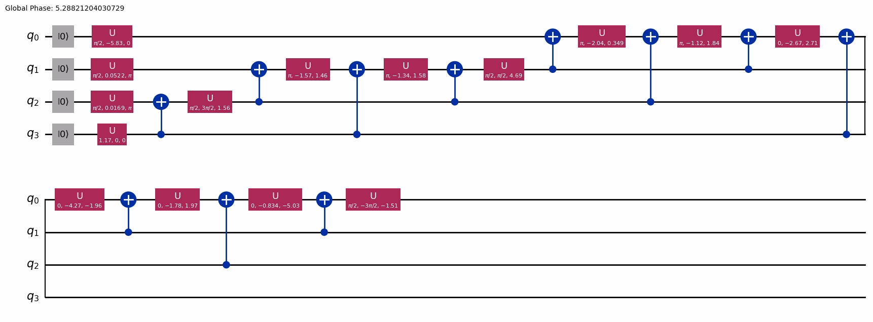
כדוגמה, בוא נקודד את הוקטור הראשון במערך הנתונים לדוגמה שלנו $\text{X}_\text{ex}$, $\vec{x}^{(1)} = (4,8,5)$ באמצעות קידוד אמפליטודה. נורמליזציה של הוקטור המתקבל נותנת לנו:

$$\sum_{i=1}^N \left|x^{(1)}_i\right|^2 = 4^2+8^2+5^2 = 105 = \left|\alpha\right|^2 \rightarrow \alpha = \sqrt{105}$$

והמצב הקוונטי של 2 Qubitים המתקבל יהיה:

$$|\psi(\vec{x}^{(1)})\rangle = \frac{1}{\sqrt{105}}(4|00\rangle+8|01\rangle+5|10\rangle+0|11\rangle)$$

בדוגמה לעיל, מספר התכונות בוקטור $N=3$ אינו חזקה של 2. כאשר $N$ אינו חזקה של 2, פשוט בוחרים ערך למספר ה-Qubitים $n$ כך ש-$2^n\geq N$ וממלאים את וקטור האמפליטודה בקבועים לא אינפורמטיביים (כאן, אפס).

כמו בקידוד בסיס, לאחר שחישבנו איזה מצב יקודד את מערך הנתונים שלנו, ב-Qiskit אנו יכולים להשתמש בפונקציה initialize להכנתו:

import math

desired_state = [
    1 / math.sqrt(105) * 4,
    1 / math.sqrt(105) * 8,
    1 / math.sqrt(105) * 5,
    1 / math.sqrt(105) * 0,
]

qc = QuantumCircuit(2)
qc.initialize(desired_state, [0, 1])

qc.decompose(reps=5).draw(output="mpl")

יתרון של קידוד אמפליטודה הוא הדרישה הנ"ל ל-$\mathrm{log}_2(N)$ Qubitים בלבד לקידוד. עם זאת, האלגוריתמים הבאים חייבים לפעול על האמפליטודות של מצב קוונטי, ושיטות להכנה ומדידה של מצבים קוונטיים אינן נוטות להיות יעילות.

בדוק את הבנתך

קרא את השאלות למטה, חשוב על תשובותיך, ולאחר מכן לחץ על המשולשים לחשיפת הפתרונות.

רשום את המצב המנורמל לקידוד הוקטור הבא (המורכב משני וקטורים ממערך הנתונים לדוגמה שלנו):

$\vec{x}=(9,8,6,2,9,2)$

באמצעות קידוד אמפליטודה.

תשובה:

כדי לקודד 6 מספרים, נצטרך לפחות 6 מצבים זמינים שעל אמפליטודותיהם נוכל לקודד. זה ידרוש 3 Qubitים. באמצעות גורם נורמליזציה לא ידוע $\alpha$, נוכל לכתוב זאת כ:

$$|\psi\rangle = \alpha(9|000\rangle+8|001\rangle+6|010\rangle+2|011\rangle+9|100\rangle+2|101\rangle+0|110\rangle+0|111\rangle)$$

שים לב ש

$$\langle \psi|\psi\rangle = |\alpha|^2\times(9^2+8^2+6^2+2^2+9^2+2^2+0^2+0^2) = |\alpha|^2\times(270)=1 \rightarrow \alpha = \frac{1}{\sqrt{270}}$$

אז לבסוף,

$$|\psi\rangle = \frac{1}{\sqrt{270}}(9|000\rangle+8|001\rangle+6|010\rangle+2|011\rangle+9|100\rangle+2|101\rangle+0|110\rangle+0|111\rangle)$$

עבור אותו וקטור נתונים $\vec{x}=(9,8,6,2,9,2),$ כתוב קוד ליצירת Circuit הטוען תכונות נתונים אלה באמצעות קידוד אמפליטודה.

תשובה:

desired_state = [
    9 / math.sqrt(270),
    8 / math.sqrt(270),
    6 / math.sqrt(270),
    2 / math.sqrt(270),
    9 / math.sqrt(270),
    2 / math.sqrt(270),
    0,
    0,
]

print(desired_state)

qc = QuantumCircuit(3)
qc.initialize(desired_state, [0, 1, 2])
qc.decompose(reps=8).draw(output="mpl")

[0.5477225575051662, 0.48686449556014766, 0.36514837167011077, 0.12171612389003691, 0.5477225575051662, 0.12171612389003691, 0, 0]

ייתכן שתצטרך להתמודד עם וקטורי נתונים גדולים מאוד. שקול את הוקטור

$$\vec{x}=(4,8,5,9,8,6,2,9,2,5,7,0,3,7,5).$$

כתוב קוד לאוטומציה של הנורמליזציה, וצור Circuit קוונטי לקידוד אמפליטודה.

תשובה:

יש תשובות אפשריות רבות. הנה קוד שמדפיס כמה שלבים בדרך:

import numpy as np
from math import sqrt

init_list = [4, 8, 5, 9, 8, 6, 2, 9, 2, 5, 7, 0, 3, 7, 5]
qubits = round(np.log(len(init_list)) / np.log(2) + 0.4999999999)
need_length = 2**qubits
pad = need_length - len(init_list)
for i in range(0, pad):
    init_list.append(0)

init_array = np.array(init_list)  # Unnormalized data vector
length = sqrt(
    sum(init_array[i] ** 2 for i in range(0, len(init_array)))
)  # Vector length
norm_array = init_array / length  # Normalized array
print("Normalized array:")
print(norm_array)
print()

qubit_numbers = []
for i in range(0, qubits):
    qubit_numbers.append(i)
print(qubit_numbers)

qc = QuantumCircuit(qubits)
qc.initialize(norm_array, qubit_numbers)
qc.decompose(reps=7).draw(output="mpl")

Normalized array: [0.17342199 0.34684399 0.21677749 0.39019949 0.34684399 0.26013299 0.086711 0.39019949 0.086711 0.21677749 0.30348849 0. 0.1300665 0.30348849 0.21677749 0. ]

[0, 1, 2, 3]

האם אתה רואה יתרונות לקידוד אמפליטודה על פני קידוד בסיס? אם כן, הסבר.

תשובה:

ייתכנו מספר תשובות. תשובה אחת היא שבהינתן הסדר הקבוע של מצבי הבסיס, קידוד האמפליטודה הזה שומר על סדר המספרים המקודדים. לעיתים קרובות הוא גם יהיה מקודד בצפיפות רבה יותר.

יתרון של קידוד אמפליטודה הוא שנדרשים רק $\log_2(N)$ Qubitים עבור וקטור נתונים $N$-ממדי ($N$-תכונות) $\vec{x}\rightarrow|\vec{x}\rangle$. עם זאת, קידוד אמפליטודה הוא בדרך כלל הליך לא יעיל הדורש הכנת מצב שרירותי, שהיא אקספוננציאלית במספר שערי CNOT. אחרת, לסיכום הכנת המצב יש מורכבות זמן ריצה פולינומית של $\mathcal O(N)$ במספר הממדים, כאשר $N = 2^n$ ו-$n$ הוא מספר ה-Qubitים. קידוד אמפליטודה "מספק חיסכון אקספוננציאלי במרחב במחיר של עלייה אקספוננציאלית בזמן"[3]; עם זאת, הגדלת זמן הריצה ל-$\mathcal O(\log N)$ ניתנת להשגה במקרים מסוימים[4]. לצורך האצה קוונטית מקצה לקצה, יש לקחת בחשבון את מורכבות זמן הריצה של טעינת הנתונים.

קידוד זווית

קידוד זווית הוא בעל עניין רב במודלי QML רבים המשתמשים במפות תכונות פאולי כמו מכונות וקטור תמיכה קוונטיות (QSVM) ומעגלים קוונטיים וריאציוניים (VQC), בין היתר. קידוד זווית קשור קשר הדוק לקידוד פאזה ולקידוד זווית צפוף המוצגים להלן. כאן נשתמש ב"קידוד זווית" כדי להתייחס לסיבוב ב-$\theta$, כלומר סיבוב מציר ה-$z$ שמתבצע למשל על ידי שער $R_X$ או שער $R_Y$[1,3]. למעשה, ניתן לקדד נתונים בכל סיבוב או שילוב של סיבובים. אך $R_Y$ נפוץ בספרות, ולכן אנו מדגישים אותו כאן.

כשמוחלים על Qubit יחיד, קידוד הזווית מעניק סיבוב בציר ה-Y שפרופורציונלי לערך הנתון. נביט בקידוד של תכונה בודדת (ה-$k^\text{th}$) מוקטור הנתונים ה-$j^\text{th}$ בסט נתונים, $\vec{x}^{(j)}_k$:

$$|\vec{x}^{(j)}_k\rangle = R_Y(\theta=\vec{x}^{(j)}_k)|0\rangle = \textstyle\cos\left(\frac{\vec{x}^{(j)}_k}{2}\right)|0\rangle + \sin\left(\frac{\vec{x}^{(j)}_k}{2}\right)|1\rangle.$$

לחלופין, ניתן לבצע קידוד זווית באמצעות שערי $R_X(\theta)$, אם כי למצב המקודד יהיה פאזה יחסית מרוכבת בהשוואה ל-$R_Y(\theta)$.

קידוד זווית שונה משתי השיטות הקודמות שנדונו בכמה דרכים. בקידוד זווית:

• כל ערך תכונה ממופה ל-Qubit מתאים, $\vec{x}^{(j)}_k \rightarrow Q_k$, ומשאיר את ה-Qubit במצב מכפלה.
• ערך מספרי אחד מקודד בכל פעם, ולא קבוצת תכונות שלמה מנקודת נתונים.
• נדרשים $n$ Qubit עבור $N$ תכונות נתונים, כאשר $n\leq N$. לרוב מתקיימת שוויון כאן. נראה כיצד $n<N$ אפשרי בסעיפים הבאים.
• ה-Circuit המתקבל הוא בעומק קבוע (בדרך כלל העומק הוא 1 לפני ה-Transpiler).

ה-Circuit הקוונטי בעומק קבוע הופך אותו לנוח במיוחד לחומרת קוונטים נוכחית. תכונה נוספת של קידוד הנתונים שלנו באמצעות $\theta$ (ובפרט, בחירתנו להשתמש בקידוד זווית ציר-Y) היא שהוא יוצר מצבים קוונטיים בעלי ערכים ממשיים שיכולים להיות שימושיים עבור יישומים מסוימים. לסיבוב ציר-Y, נתונים ממופים עם שער סיבוב ציר-Y $R_Y(\theta)$ בזווית ממשית $\theta \in (0, 2\pi]$ (Qiskit RYGate). כמו בקידוד פאזה (ראה להלן), אנו ממליצים לשנות קנה מידה לנתונים כך ש-$\vec{x}^{(j)}_k \in (0,2\pi]$, כדי למנוע אובדן מידע ותופעות לא רצויות אחרות.

קוד Qiskit הבא מסובב Qubit יחיד ממצב ראשוני $|0\rangle$ כדי לקדד ערך נתון $\vec{x}^{(j)}_k=\frac{1}{2}\pi$.

from qiskit.quantum_info import Statevector
from math import pi

qc = QuantumCircuit(1)
state1 = Statevector.from_instruction(qc)
qc.ry(pi / 2, 0)  # Phase gate rotates by an angle pi/2
state2 = Statevector.from_instruction(qc)
states = state1, state2

נגדיר פונקציה להצגה חזותית של הפעולה על וקטור המצב. פרטי הגדרת הפונקציה אינם חשובים, אך היכולת להמחיש את וקטורי המצב ושינוייהם היא חשובה.

import numpy as np
from qiskit.visualization.bloch import Bloch
from qiskit.visualization.state_visualization import _bloch_multivector_data

def plot_Nstates(states, axis, plot_trace_points=True):
    """This function plots N states to 1 Bloch sphere"""
    bloch_vecs = [_bloch_multivector_data(s)[0] for s in states]

    if axis is None:
        bloch_plot = Bloch()
    else:
        bloch_plot = Bloch(axes=axis)

    bloch_plot.add_vectors(bloch_vecs)

    if len(states) > 1:

        def rgba_map(x, num):
            g = (0.95 - 0.05) / (num - 1)
            i = 0.95 - g * num
            y = g * x + i
            return (0.0, y, 0.0, 0.7)

        num = len(states)
        bloch_plot.vector_color = [rgba_map(x, num) for x in range(1, num + 1)]

    bloch_plot.vector_width = 3
    bloch_plot.vector_style = "simple"

    if plot_trace_points:

        def trace_points(bloch_vec1, bloch_vec2):
            # bloch_vec = (x,y,z)
            n_points = 15
            thetas = np.arccos([bloch_vec1[2], bloch_vec2[2]])
            phis = np.arctan2(
                [bloch_vec1[1], bloch_vec2[1]], [bloch_vec1[0], bloch_vec2[0]]
            )
            if phis[1] < 0:
                phis[1] = phis[1] + 2 * pi
            angles0 = np.linspace(phis[0], phis[1], n_points)
            angles1 = np.linspace(thetas[0], thetas[1], n_points)

            xp = np.cos(angles0) * np.sin(angles1)
            yp = np.sin(angles0) * np.sin(angles1)
            zp = np.cos(angles1)
            pnts = [xp, yp, zp]
            bloch_plot.add_points(pnts)
            bloch_plot.point_color = "k"
            bloch_plot.point_size = [4] * len(bloch_plot.points)
            bloch_plot.point_marker = ["o"]

        for i in range(len(bloch_vecs) - 1):
            trace_points(bloch_vecs[i], bloch_vecs[i + 1])

    bloch_plot.sphere_alpha = 0.05
    bloch_plot.frame_alpha = 0.15
    bloch_plot.figsize = [4, 4]

    bloch_plot.render()

plot_Nstates(states, axis=None, plot_trace_points=True)

זו הייתה רק תכונה בודדת של וקטור נתונים יחיד. כשמקודדים $N$ תכונות לזוויות הסיבוב של $n$ Qubit, נניח עבור וקטור הנתונים ה-$j^\text{th}$ $\vec{x}^{(j)} = (x_1,...,x_N),$ מצב המכפלה המקודד ייראה כך:

$$|\vec{x}^{(j)}\rangle = \bigotimes^N_{k=1} \cos(\vec{x}^{(j)}_k)|0\rangle + \sin(\vec{x}^{(j)}_k)|1\rangle$$

נציין שזה שקול ל-

$$|\vec{x}^{(j)}\rangle = \bigotimes^N_{k=1} R_Y(2\vec{x}^{(j)}_k)|0\rangle.$$

בדוק את הבנתך

קרא את השאלות הבאות, חשוב על תשובותיך, ולאחר מכן לחץ על המשולשים לחשיפת הפתרונות.

קדד את וקטור הנתונים $\vec{x} = (0, \pi/4, \pi/2)$ באמצעות קידוד זווית, כפי שתואר לעיל.

תשובה:

qc = QuantumCircuit(3)
qc.ry(0, 0)
qc.ry(2 * math.pi / 4, 1)
qc.ry(2 * math.pi / 2, 2)
qc.draw(output="mpl")

בשימוש בקידוד זווית כפי שתואר לעיל, כמה Qubit נדרשים לקידוד 5 תכונות?

תשובה: 5

קידוד פאזה

קידוד פאזה דומה מאוד לקידוד הזווית שתואר לעיל. זווית הפאזה של Qubit היא זווית ממשית $\phi$ סביב ציר ה-$z$ מציר ה-+$x$. נתונים ממופים עם סיבוב פאזה, $P(\phi) = e^{i\phi/2}R_Z(\phi)$, כאשר $\phi \in (0,2\pi]$ (ראה Qiskit PhaseGate למידע נוסף). מומלץ לשנות קנה מידה לנתונים כך ש-$\vec{x}^{(j)}_k \in (0,2\pi]$. זה מונע אובדן מידע ותופעות לא רצויות אחרות[1,2].

Qubit מאותחל לרוב במצב $|0\rangle$, שהוא eigenvector של אופרטור סיבוב הפאזה, כלומר מצב ה-Qubit צריך קודם להיות מסובב כדי שקידוד הפאזה יוכל להיות מיושם. לכן הגיוני לאתחל את המצב עם שער הדמארד: $H|0\rangle = |+\rangle = \textstyle\frac{1}{\sqrt{2}}(|0\rangle + |1\rangle)$. קידוד פאזה על Qubit יחיד פירושו הענקת פאזה יחסית פרופורציונלית לערך הנתון:

$$|\vec{x}^{(j)}_k\rangle = P(\phi=\vec{x}^{(j)}_k)|+\rangle = \textstyle\frac{1}{\sqrt{2}}\big(|0\rangle + e^{i\vec{x}^{(j)}_k}|1\rangle\big).$$

פרוצדורת קידוד הפאזה ממפה כל ערך תכונה לפאזה של Qubit מתאים, $\vec{x}^{(j)}_k \rightarrow Q_k$. בסך הכל, לקידוד פאזה יש עומק Circuit של 2, כולל שכבת הדמארד, מה שהופך אותו לסכמת קידוד יעילה. מצב רב-Qubit המקודד בפאזה ($n$ Qubit עבור $N=n$ תכונות) הוא מצב מכפלה:

$$|\vec{x}^{(j)}\rangle = \bigotimes_{k=1}^{N} P_k(\phi = \vec{x}^{(j)}_k)|+\rangle^{\otimes N} = {\textstyle\frac{1}{\sqrt{2^N}}} \bigotimes_{k=1}^{N}\big(|0\rangle + e^{i\vec{x}^{(j)}_k}|1\rangle\big).$$

קוד Qiskit הבא מכין תחילה את המצב הראשוני של Qubit יחיד על ידי סיבובו עם שער הדמארד, ולאחר מכן מסובב אותו שוב באמצעות שער פאזה כדי לקדד תכונת נתון $\vec{x}^{(j)}_k=\frac{1}{2}\pi$.

qc = QuantumCircuit(1)
qc.h(0)  # Hadamard gate rotates state down to Bloch equator
state1 = Statevector.from_instruction(qc)

qc.p(pi / 2, 0)  # Phase gate rotates by an angle pi/2
state2 = Statevector.from_instruction(qc)

states = state1, state2

qc.draw("mpl", scale=1)

נוכל להמחיש את הסיבוב ב-$\phi$ באמצעות פונקציית plot_Nstates שהגדרנו.

plot_Nstates(states, axis=None, plot_trace_points=True)

תרשים כדור הבלוך מראה את סיבוב ציר ה-Z $|+\rangle \rightarrow P(\frac{1}{2}\pi)|+\rangle$ כאשר $\vec{x}^{(j)}_k=\frac{1}{2}\pi$. החץ הירוק הבהיר מראה את המצב הסופי.

קידוד פאזה משמש במפות תכונות קוונטיות רבות, בפרט מפות תכונות $Z$ ו-$ZZ$, ומפות תכונות פאולי כלליות, בין היתר.

בדוק את הבנתך

קרא את השאלות הבאות, חשוב על תשובותיך, ולאחר מכן לחץ על המשולשים לחשיפת הפתרונות.

כמה Qubit נדרשים כדי להשתמש בקידוד פאזה כפי שתואר לעיל לאחסון 8 תכונות?

תשובה: 8

כתוב קוד לטעינת הוקטור $\vec{x}^{(1)}=(4,8,5,9,8,6,2,9,2,5,7,0)$ באמצעות קידוד פאזה.

תשובה:

ייתכנו תשובות רבות. הנה דוגמה אחת:

phase_data = [4, 8, 5, 9, 8, 6, 2, 9, 2, 5, 7, 0]
qc = QuantumCircuit(len(phase_data))
for i in range(0, len(phase_data)):
    qc.h(i)
    qc.rz(phase_data[i] * 2 * math.pi / float(max(phase_data)), i)
qc.draw(output="mpl")

קידוד זווית צפוף

קידוד זווית צפוף (DAE) הוא שילוב של קידוד זווית וקידוד פאזה. DAE מאפשר לקדד שני ערכי תכונות ב-Qubit יחיד: אחד עם זווית סיבוב ציר-Y, והשני עם זווית סיבוב ציר-$z$: $\vec{x}^{(j)}_k,$ $\vec{x}^{(j)}_\ell \rightarrow \theta, \phi$. הוא מקדד שתי תכונות כדלקמן:

$$|\vec{x}^{(j)}_k,\vec{x}^{(j)}_\ell\rangle = R_Z(\phi=\vec{x}^{(j)}_\ell) R_Y(\theta=\vec{x}^{(j)}_k)|0\rangle = \cos\left(\frac{\vec{x}^{(j)}_k}{2}\right)|0\rangle + e^{i\vec{x}^{(j)}_\ell} \sin\left(\frac{\vec{x}^{(j)}_k}{2}\right)|1\rangle.$$

קידוד שתי תכונות נתונים ל-Qubit אחד מביא לצמצום של פי $2\times$ במספר ה-Qubit הנדרשים לקידוד. בהרחבה לתכונות נוספות, ניתן לקדד את וקטור הנתונים $\vec{x} = (x_1,...,x_N)$ כ:

$$|\vec{x}\rangle = \bigotimes_{k=1}^{N/2} \cos(x_{2k-1})|0\rangle + e^{i x_{2k}}\sin(x_{2k-1})|1\rangle$$

ניתן להכליל את DAE לפונקציות שרירותיות של שתי התכונות במקום הפונקציות הסינוסואידיות שבשימוש כאן. זה נקרא קידוד Qubit כללי[7].

כדוגמה ל-DAE, הקוד שלהלן מקדד ומדמה את הקידוד של התכונות $x_1=\theta = 3\pi/8$ ו-$x_2=\phi = 7\pi/4$.

qc = QuantumCircuit(1)
state1 = Statevector.from_instruction(qc)
qc.ry(3 * pi / 8, 0)
state2 = Statevector.from_instruction(qc)
qc.rz(7 * pi / 4, 0)
state3 = Statevector.from_instruction(qc)
states = state1, state2, state3

plot_Nstates(states, axis=None, plot_trace_points=True)

בדוק את הבנתך

קרא את השאלות הבאות, חשוב על תשובותיך, ולאחר מכן לחץ על המשולשים לחשיפת הפתרונות.

בהתאם לטיפול לעיל, כמה Qubit נדרשים לקידוד 6 תכונות באמצעות קידוד צפוף?

תשובה: 3

כתוב קוד לטעינת הוקטור $\vec{x}^{(1)}=(4,8,5,9,8,6,2,9,2,5,7,0,3,7,5)$ באמצעות קידוד זווית צפוף.

תשובה:

שים לב שהרחבנו את הרשימה ב-"0" כדי להימנע מבעיית פרמטר בלתי מנוצל יחיד בסכמת הקידוד שלנו.

dense_data = [4, 8, 5, 9, 8, 6, 2, 9, 2, 5, 7, 0, 3, 7, 5, 0]
qc = QuantumCircuit(int(len(dense_data) / 2))
entry = 0
for i in range(0, int(len(dense_data) / 2)):
    qc.ry(dense_data[entry] * 2 * math.pi / float(max(dense_data)), i)
    entry = entry + 1
    qc.rz(dense_data[entry] * 2 * math.pi / float(max(dense_data)), i)
    entry = entry + 1
qc.draw(output="mpl")

קידוד עם מפות פיצ'רים מובנות

קידוד בנקודות שרירותיות

קידוד זוויתי, קידוד פאזה וקידוד צפוף הכינו מצבי מכפלה עם פיצ'ר מקודד על כל Qubit (או שני פיצ'רים לכל Qubit). זה שונה מקידוד בסיס וקידוד אמפליטודה, שבהם מנצלים מצבים שזורים. אין התאמה 1:1 בין פיצ'ר נתונים ל-Qubit. בקידוד אמפליטודה, למשל, ייתכן שפיצ'ר אחד הוא האמפליטודה של המצב $|01\rangle$ ופיצ'ר אחר הוא האמפליטודה של $|10\rangle$. בדרך כלל, שיטות שמקודדות במצבי מכפלה מניבות Circuit-ים רדודים יותר ויכולות לאחסן 1 או 2 פיצ'רים על כל Qubit. שיטות שמשתמשות בשזירה ומשייכות פיצ'ר למצב ולא ל-Qubit מובילות ל-Circuit-ים עמוקים יותר, ויכולות לאחסן יותר פיצ'רים לכל Qubit בממוצע.

אך הקידוד לא חייב להיות כולו במצבי מכפלה או כולו במצבים שזורים כמו בקידוד אמפליטודה. למעשה, ערכות קידוד רבות המובנות ב-Qiskit מאפשרות קידוד גם לפני וגם אחרי שכבת שזירה, בניגוד להתחלה בלבד. זה ידוע בשם "העלאה מחדש של נתונים" (data reuploading). לעבודות קשורות, ראו הפניות [5] ו-[6].

בחלק זה נשתמש ונמחיש כמה מערכות הקידוד המובנות. כל השיטות בחלק זה מקודדות $N$ פיצ'רים כסיבובים על $N$ Gate-ים עם פרמטרים על $n$ Qubit-ים, כאשר $n \leq N$. שימו לב שמקסום טעינת נתונים לכמות Qubit-ים נתונה אינו השיקול היחיד. במקרים רבים, עומק ה-Circuit עשוי להיות שיקול חשוב אפילו יותר ממספר ה-Qubit-ים.

Efficient SU2

דוגמה נפוצה ושימושית לקידוד עם שזירה היא ה-Circuit efficient_su2 של Qiskit. מדהים לציין שה-Circuit הזה יכול, למשל, לקודד 8 פיצ'רים על 2 Qubit-ים בלבד. בואו נראה זאת, ואז ננסה להבין כיצד זה אפשרי.

from qiskit.circuit.library import efficient_su2

circuit = efficient_su2(num_qubits=2, reps=1, insert_barriers=True)
circuit.decompose().draw(output="mpl")

כשנכתוב את המצב שלנו, נשתמש בקונבנציית Qiskit שלפיה Qubit-ים בעלי המשקל הנמוך ביותר מסודרים בצד ימין, כמו $|q_2,q_1,q_0\rangle$ או $|q_2\rangle\otimes|q_1\rangle\otimes|q_0\rangle.$ מצבים אלו יכולים להיות מורכבים מאוד מהר מאוד, ודוגמה נדירה זו עשויה להסביר מדוע מצבים כאלה לעתים נדירות נכתבים במפורש.

המערכת שלנו מתחילה במצב $|00\rangle.$ עד המחסום הראשון (נקודה שנסמן כ-$b1$), המצבים שלנו הם:

$$|\psi\rangle_{b1} = \left(\cos\left(\frac{\theta_1}{2}\right)|0\rangle+\sin\left(\frac{\theta_1}{2}\right)e^{i\theta_3}|1\rangle\right)\otimes\left(\cos\left(\frac{\theta_0}{2}\right)|0\rangle+\sin\left(\frac{\theta_0}{2}\right)e^{i\theta_2}|1\rangle\right)$$

זה בדיוק קידוד צפוף, שכבר ראינו. עכשיו אחרי שער ה-CNOT, במחסום השני ($b2$), המצב שלנו הוא

$$\begin{aligned} |\psi\rangle_{b2} = & \cos\left(\frac{\theta_1}{2}\right)\cos\left(\frac{\theta_0}{2}\right)|00\rangle+\cos\left(\frac{\theta_1}{2}\right)\sin\left(\frac{\theta_0}{2}\right)e^{i\theta_2}|11\rangle\\ + & \sin\left(\frac{\theta_1}{2}\right)\cos\left(\frac{\theta_0}{2}\right)e^{i\theta_3}|10\rangle+\sin\left(\frac{\theta_1}{2}\right)\sin\left(\frac{\theta_0}{2}\right)e^{i\theta_2}e^{i\theta_3}|01\rangle \end{aligned}$$

כעת נפעיל את סט הסיבובים האחרון על Qubit יחיד ונאסוף מצבים דומים כדי לקבל:

$$\begin{align*} |\psi\rangle_{\text{final}} = & \left[\cos\left(\frac{\theta_0}{2}\right)\left(\cos\left(\frac{\theta_1}{2}\right)\cos\left(\frac{\theta_5}{2}\right)-\sin\left(\frac{\theta_1}{2}\right)\sin\left(\frac{\theta_5}{2}\right)e^{i\theta_3}\right)\cos\left(\frac{\theta_4}{2}\right)\right.\\ + & \left.\sin\left(\frac{\theta_0}{2}\right)\left(\cos\left(\frac{\theta_1}{2}\right)\sin\left(\frac{\theta_5}{2}\right)-\sin\left(\frac{\theta_1}{2}\right)\cos\left(\frac{\theta_5}{2}\right)e^{i\theta_3}\right)\sin\left(\frac{\theta_4}{2}\right)e^{i\theta_2}\right] |00\rangle\\ + & \left[\cos\left(\frac{\theta_0}{2}\right)\left(\cos\left(\frac{\theta_1}{2}\right)\cos\left(\frac{\theta_5}{2}\right)-\sin\left(\frac{\theta_1}{2}\right)\sin\left(\frac{\theta_5}{2}\right)e^{i\theta_3}\right)\sin\left(\frac{\theta_4}{2}\right)\right.\\ + & \left.\sin\left(\frac{\theta_0}{2}\right)\left(-\cos\left(\frac{\theta_1}{2}\right)\sin\left(\frac{\theta_5}{2}\right)+\sin\left(\frac{\theta_1}{2}\right)\cos\left(\frac{\theta_5}{2}\right)e^{i\theta_3}\right)\cos\left(\frac{\theta_4}{2}\right)e^{i\theta_2}\right] e^{i\theta_6}|01\rangle\\ + & \left[\cos\left(\frac{\theta_0}{2}\right)\left(\cos\left(\frac{\theta_1}{2}\right)\sin\left(\frac{\theta_5}{2}\right)+\sin\left(\frac{\theta_1}{2}\right)\cos\left(\frac{\theta_5}{2}\right)e^{i\theta_3}\right)\cos\left(\frac{\theta_4}{2}\right)\right.\\ - & \left.\sin\left(\frac{\theta_0}{2}\right)\left(\cos\left(\frac{\theta_1}{2}\right)\cos\left(\frac{\theta_5}{2}\right)+\sin\left(\frac{\theta_1}{2}\right)\sin\left(\frac{\theta_5}{2}\right)e^{i\theta_3}\right)\sin\left(\frac{\theta_4}{2}\right)e^{i\theta_2}\right] e^{i\theta_7}|10\rangle\\ + & \left[\cos\left(\frac{\theta_0}{2}\right)\left(\cos\left(\frac{\theta_1}{2}\right)\sin\left(\frac{\theta_5}{2}\right)+\sin\left(\frac{\theta_1}{2}\right)\cos\left(\frac{\theta_5}{2}\right)e^{i\theta_3}\right)\sin\left(\frac{\theta_4}{2}\right)\right.\\ + & \left.\sin\left(\frac{\theta_0}{2}\right)\left(\cos\left(\frac{\theta_1}{2}\right)\cos\left(\frac{\theta_5}{2}\right)+\sin\left(\frac{\theta_1}{2}\right)\sin\left(\frac{\theta_5}{2}\right)e^{i\theta_3}\right)\cos\left(\frac{\theta_4}{2}\right)e^{i\theta_2}\right] e^{i\theta_6}e^{i\theta_7}|11\rangle \end{align*}$$

כנראה שזה מסובך מדי לניתוח. במקום זאת, פשוט עצרו ושאלו: כמה פרמטרים טענו אל המצב? שמונה. אבל יש לנו רק ארבעה מצבי בסיס חישוביים. במבט ראשון עלול להיראות שטענו יותר פרמטרים ממה שהגיוני, שכן את המצב הסופי ניתן לכתוב כ-$\psi_\text{final} = c_0|00\rangle+c_1|01\rangle+c_2|10\rangle+c_3|11\rangle$. שימו לב, עם זאת, שכל מקדם הוא מרוכב! כשכותבים כך:

$$\psi_\text{final} = (a_0+ib_0)|00\rangle+(a_1+ib_1)|01\rangle+(a_2+ib_2)|10\rangle+(a_3+ib_3)|11\rangle$$

רואים שאכן יש לנו שמונה פרמטרים במצב שעליהם ניתן לקודד את שמונת הפיצ'רים שלנו.

על ידי הגדלת מספר ה-Qubit-ים והגדלת מספר החזרות של שכבות השזירה והסיבוב, ניתן לקודד הרבה יותר נתונים. כתיבת פונקציות הגל הופכת לבלתי אפשרית מהר מאוד. אבל עדיין ניתן לראות את הקידוד בפעולה. כאן אנחנו מקודדים את וקטור הנתונים $\vec{x}$ עם 12 פיצ'רים, על Circuit של efficient_su2 עם 3 Qubit-ים, תוך שימוש בכל אחד מה-Gate-ים עם פרמטרים לקידוד פיצ'ר שונה.

$$\vec{x} = (0.1,0.2,0.3,0.4,0.5,0.6,0.7,0.8,0.9,1.0,1.1,1.2)$$

בוקטור נתונים זה, הפיצ'רים מוצגים בסדר מסוים. בפני עצמו, לא משנה אם הם מקודדים בסדר הזה או בסדר הפוך. מה שחשוב הוא לעקוב אחרי הסדר ולהיות עקביים. שימו לב בתרשים ה-Circuit ש-efficient_su2 מניח סדר קידוד מסוים, ספציפית מלא את שכבת ה-Gate-ים הראשונה מ-Qubit 0 עד Qubit 2, ולאחר מכן עובר לשכבה הבאה. זה לא עקבי ולא לא-עקבי עם ייצוג little-endian, שכן כאן לא ניתן לסדר את פיצ'רי הנתונים לפי Qubit מראש, לפני שנקבע Circuit קידוד.

x = [0.1, 0.2, 0.3, 0.4, 0.5, 0.6, 0.7, 0.8, 0.9, 1.0, 1.1, 1.2]
circuit = efficient_su2(num_qubits=3, reps=1, insert_barriers=True)
encode = circuit.assign_parameters(x)
encode.decompose().draw(output="mpl")

במקום להגדיל את מספר ה-Qubit-ים, אפשר לבחור להגדיל את מספר החזרות של שכבות השזירה והסיבוב. אבל יש גבולות לכמות החזרות שיש בהן תועלת. כפי שצוין קודם, יש פשרה: Circuit-ים עם יותר Qubit-ים או יותר חזרות של שכבות שזירה וסיבוב עשויים לאחסן יותר פרמטרים, אך עושים זאת עם עומק Circuit גדול יותר. נחזור לעומק של כמה מפות פיצ'רים מובנות בהמשך. מספר שיטות הקידוד הבאות המובנות ב-Qiskit כוללות "מפת פיצ'רים" בשמותיהן. כדאי להדגיש שוב שקידוד נתונים ל-Circuit קוונטי הוא מיפוי פיצ'רים, במובן שהוא לוקח נתונים למרחב חדש: מרחב הילברט של ה-Qubit-ים המעורבים. הקשר בין הממדיות של מרחב הפיצ'רים המקורי לבין מרחב הילברט יהיה תלוי ב-Circuit שבו משתמשים לקידוד.

מפת פיצ'רים $Z$

מפת פיצ'רים $Z$ (ZFM) ניתנת לפירוש כהרחבה טבעית של קידוד הפאזה. ה-ZFM מורכבת משכבות מתחלפות של Gate-ים על Qubit יחיד: שכבות Gate של Hadamard ושכבות Gate של פאזה. נניח שוקטור הנתונים $\vec{x}$ כולל $N$ פיצ'רים. ה-Circuit הקוונטי שמבצע את מיפוי הפיצ'רים מיוצג כאופרטור אוניטרי שפועל על המצב ההתחלתי:

$$\mathscr{U}_{\text{ZFM}}(\vec{x})|0\rangle^{\otimes N}=|\phi(\vec{x})\rangle$$

כאשר $|0\rangle^{\otimes N}$ הוא מצב הבסיס של $N$ Qubit-ים. סימון זה משמש לעקביות עם הפניה [4] של Havlicek et al. פיצ'רי הנתונים $x_i$ מועברים בהתאמה 1:1 לQubit-ים התואמים. לדוגמה, אם יש לכם 8 פיצ'רים בוקטור נתונים, תשתמשו ב-8 Qubit-ים. ה-Circuit של ZFM מורכב מ-$r$ חזרות של תת-Circuit הכולל שכבות Gate של Hadamard ושכבות Gate של פאזה. שכבת Hadamard מורכבת מ-Gate של Hadamard הפועל על כל Qubit ברגיסטר של $n$ Qubit-ים, $H \otimes H \otimes \dots \otimes H = H^{\otimes n}$, באותו שלב של האלגוריתם. תיאור זה חל גם על שכבת Gate של פאזה שבה ה-Qubit ה-$i$ נפעל על ידי $P(\vec{x}_i)$. לכל Gate מסוג $P$ יש פיצ'ר אחד כארגומנט, אך שכבת Gate הפאזה ($P(\vec{x}_1)\otimes\ldots P(\vec{x}_k)\otimes\ldots P(\vec{x}_N)$) היא פונקציה של וקטור הנתונים. ה-Circuit האוניטרי המלא של ZFM עם חזרה יחידה הוא:

$$\mathscr{U}_{\text{ZFM}}=\big(P(\vec{x}_1)\otimes\ldots P(\vec{x}_k)\otimes\ldots P(\vec{x}_N)H^{\otimes N}\big)=\left(\bigotimes_{k = 1}^N P(\vec{x}_k)\right)H^{\otimes N}$$

ואז $r$ חזרות של אוניטרי זה יהיו

$$\mathscr{U}^{(r)}_{\text{ZFM}}\left(\vec{x}\right)=\prod_{s=1}^{r}\left[\left(\bigotimes_{k = 1}^N P(\vec{x}_k)\right)H^{\otimes N}\right]$$

פיצ'רי הנתונים, $x_k$, ממופים ל-Gate-ים של פאזה באותו אופן בכל $r$ החזרות. מצב מפת הפיצ'רים ZFM הוא מצב מכפלה ויעיל לסימולציה קלאסית[4].

לדוגמה קטנה להתחלה, Circuit של ZFM עם שני Qubit-ים מקודד באמצעות Qiskit ומצויר כדי להציג את מבנה ה-Circuit הפשוט. בדוגמה, חזרה יחידה, $r=1$, מיושמת עם וקטור הנתונים $\vec{x} = \left(\textstyle\frac{1}{2}\pi, \textstyle\frac{1}{3}\pi\right)$. שימו לב שזה כתוב בסדר הסטנדרטי של וקטור ב-Python, כלומר האיבר ה-$0$ הוא $\textstyle\frac{1}{2}\pi.$ אנחנו חופשיים לקודד פיצ'ר ה-$0$ הזה על ה-Qubit ה-$0$ שלנו, או על ה-$N$. שוב, לא תמיד ניתן לקבוע מיפוי 1:1 יחיד מסדר פיצ'רים לסדר Qubit-ים, שכן מפות פיצ'רים שונות מקודדות מספר שונה של פיצ'רים לכל Qubit. שוב, מה שחשוב הוא שנהיה מודעים היכן מקודד כל פיצ'ר. כשמספקים רשימת פרמטרים למפת פיצ'רים $Z$, היא תקודד פיצ'ר 0 מהרשימה ל-Qubit בעל המשקל הנמוך ביותר עם Gate בעל פרמטר, כלומר Qubit 0. אז נפעל לפי קונבנציה זו כשעושים זאת ידנית. נקודד $\textstyle\frac{1}{2}\pi$ על ה-Qubit ה-$0$, ו-$\textstyle\frac{1}{3}\pi$ על ה-Qubit ה-$1$.

האופרטור האוניטרי של circuit ה-ZFM פועל על המצב ההתחלתי בדרך הבאה:

$$\mathscr{U}_{\text{ZFM}}(\bar{x})|00\rangle = P(\bar{x})^{\otimes 2} H^{\otimes 2}|00\rangle = \left( P\left(\textstyle\frac{1}{3}\pi\right)H|0\rangle \right) \otimes \left(P\left(\textstyle\frac{1}{2}\pi\right)H|0\rangle\right).$$

הנוסחה סודרה מחדש סביב מכפלת הטנסור כדי להדגיש את הפעולות על כל Qubit. קוד Qiskit הבא משתמש ב-Gate-ים של Hadamard ופאזה במפורש כדי להראות את מבנה ה-ZFM:

qc0 = QuantumCircuit(1)
qc1 = QuantumCircuit(1)

qc0.h(0)
qc0.p(pi / 2, 0)

qc1.h(0)
qc1.p(pi / 3, 0)

# Combine circuits qc0 and qc1 into 1 circuit
qc = QuantumCircuit(2)
qc.compose(qc0, [0], inplace=True)
qc.compose(qc1, [1], inplace=True)

qc.draw("mpl", scale=1)

כעת נקודד את אותו וקטור נתונים $\vec{x} = \left(\textstyle\frac{1}{2}\pi, \textstyle\frac{1}{3}\pi\right)$ ל-Circuit של ZFM עם שלוש חזרות, $r=3$, באמצעות מחלקת z_feature_map של Qiskit, שבסך הכל נותנת לנו את מפת הפיצ'רים הקוונטית $\mathscr{U}_{\text{ZFM}}(\vec{x})$. כברירת מחדל במחלקת z_feature_map, הפרמטרים $\beta$ מוכפלים ב-2 לפני המיפוי ל-Gate הפאזה $\beta \rightarrow P(\theta = 2\beta)$. כדי לשחזר את אותם קידודים כמו לעיל, נחלק ב-2.

from qiskit.circuit.library import z_feature_map

zfeature_map = z_feature_map(feature_dimension=2, reps=3)
zfeature_map = zfeature_map.assign_parameters([(1 / 2) * pi / 2, (1 / 2) * pi / 3])
zfeature_map.decompose().draw("mpl")

ברור שזה מיפוי שונה מזה שנעשה ידנית לעיל, אך שימו לב לעקביות בסדר הפרמטרים: $\textstyle\frac{1}{2}\pi$ קודד שוב על ה-Qubit ה-$0$.

ניתן להשתמש ב-ZFM דרך מחלקת ה-ZFM של Qiskit; ניתן גם להשתמש במבנה זה כהשראה לבניית מיפוי פיצ'רים משלכם.

מפת פיצ'רים $ZZ$

מפת פיצ'רים $ZZ$ (ZZFM) מרחיבה את ה-ZFM בהכללת Gate-ים של שזירה על שני Qubit-ים, ספציפית Gate הסיבוב $ZZ$, $R_{ZZ}(\theta)$. ה-ZZFM עצמה מוערכת כיקרה בדרך כלל לחישוב על מחשב קלאסי, בניגוד ל-ZFM.

$R_{ZZ}(\theta)$ מממש אינטראקציה $ZZ$ ומכסים מיקסום שזירה עבור $\theta = \textstyle{\frac{1}{2}}\pi$. ניתן לפרק את $R_{ZZ}(\theta)$ לסדרת Gate-ים על שני Qubit-ים, כפי שמוצג בקוד Qiskit הבא באמצעות שער RZZ ושיטת המחלקה decompose של QuantumCircuit. נקודד פיצ'ר יחיד של וקטור הנתונים $\vec{x}$: $\vec{x}_k=\pi.$

qc = QuantumCircuit(2)
qc.rzz(pi, 0, 1)
qc.draw("mpl", scale=1)

כפי שקורה לעתים קרובות, אנחנו רואים זאת מיוצג כיחידה הדומה ל-Gate יחיד, עד שמשתמשים ב-.decompose() כדי לראות את כל ה-Gate-ים המרכיבים.

qc.decompose().draw("mpl", scale=1)

הנתונים ממופים עם סיבוב פאזה $P(\theta) = e^{i\theta/2}R_Z(\theta)$ על ה-Qubit השני. שער $R_{ZZ}(\theta)$ משזר את שני ה-Qubit-ים שעליהם הוא פועל בדרגת שזירה הנקבעת על ידי ערך הפיצ'ר המקודד.

ה-Circuit המלא של ZZFM מורכב מ-Gate של Hadamard ו-Gate של פאזה, כמו ב-ZFM, ואחריהם השזירה המתוארת לעיל. חזרה יחידה של Circuit ה-ZZFM היא:

$$\mathscr{U}_{\text{ZZFM}}(\vec{x}) = U_{ZZ}(\vec{x})\big(P(\vec{x}_1)\otimes\ldots P(\vec{x}_k)\otimes\ldots P(\vec{x}_N)H^{\otimes N}\big)=U_{ZZ}(\vec{x})\left(\bigotimes_{k = 1}^N P(\vec{x}_k)\right)H^{\otimes N},$$

כאשר $U_{ZZ}(\vec{x})$ מכיל שכבת Gate-ים ZZ המובנית על ידי ערכת שזירה. מספר ערכות שזירה מוצגות בבלוקי קוד למטה. מבנה $U_{ZZ}(\vec{x})$ כולל גם פונקציה שמשלבת את פיצ'רי הנתונים מה-Qubit-ים המשוזרים בדרך הבאה. נניח שה-Gate $R_{ZZ}$ יופעל על Qubit-ים $p$ ו-$q$. בשכבת הפאזה, ל-Qubit-ים אלה יש Gate-ים של פאזה שמקודדים $\vec{x}_p$ ו-$\vec{x}_q$ עליהם, בהתאמה. הארגומנט $\theta_{q,p}$ של $R_{ZZ,q,p}(\theta_{q,p})$ לא יהיה פשוט אחד מהפיצ'רים האלה או האחר, אלא פונקציה המסומנת לרוב ב-$\phi$ (לא להתבלבל עם זווית האזימוט):

$$\theta_{q,p} \rightarrow \phi(\vec{x}_q, \vec{x}_p) = 2(\pi-\vec{x}_q)(\pi-\vec{x}_p).$$

נראה זאת בכמה דוגמאות להלן. ההרחבה למספר חזרות זהה למקרה של z_feature_map:

$$\mathscr{U}^{(r)}_{\text{ZZFM}}\left(\vec{x}\right)=\prod_{s=1}^{r}\left[U_{ZZ}(\vec{x})\left(\bigotimes_{k = 1}^N P(\vec{x}_k)\right)H^{\otimes N}\right].$$

מכיוון שהאופרטורים הפכו מורכבים יותר, בואו נקודד תחילה וקטור נתונים $\vec{x} = (x_0, x_1)$ עם ZZFM של שני Qubit-ים וחזרה אחת באמצעות הקוד הבא:

from qiskit.circuit.library import zz_feature_map

feature_dim = 2
zzfeature_map = zz_feature_map(
    feature_dimension=feature_dim, entanglement="linear", reps=1
)
zzfeature_map.decompose(reps=1).draw("mpl", scale=1)

כברירת מחדל ב-Qiskit, הפיצ'רים $(\vec{x}_1, \vec{x}_2)$ ממופים יחד ל-$R_{ZZ}(\theta)$ על ידי פונקציית המיפוי $\theta_{1,2} = \phi(\vec{x}_1, \vec{x}_2) = 2(\pi-\vec{x}_1)(\pi-\vec{x}_2)$. Qiskit מאפשרת למשתמש להתאים אישית את הפונקציה $\phi$ (או $\phi_S$ כאשר $S$ הוא קבוצת זוגות ה-Qubit-ים המקושרים דרך Gate-ים $R_{ZZ}$) כשלב עיבוד מקדים.

עוברים לוקטור נתונים בעל ארבעה ממדים $\vec{x} = (\vec{x}_1, \vec{x}_2, \vec{x}_3, \vec{x}_4)$ וממפים לZZFM עם ארבעה Qubit-ים וחזרה אחת, נוכל להתחיל לראות את המיפוי $\phi$ עבור זוגות Qubit שונים. נוכל גם לראות את המשמעות של שזירה "לינארית":

feature_dim = 4
zzfeature_map = zz_feature_map(
    feature_dimension=feature_dim, entanglement="linear", reps=1
)
zzfeature_map.decompose().draw("mpl", scale=1)

בערכת השזירה הלינארית, זוגות Qubit-ים שכנים (ממוספרים) ב-Circuit הזה משוזרים. יש ערכות שזירה מובנות אחרות ב-Qiskit, כולל circular ו-full.

מפת פיצ'רים Pauli

מפת פיצ'רים Pauli (PFM) היא הכללה של ZFM ו-ZZFM לשימוש ב-Gate-ים שרירותיים של Pauli. מפת פיצ'רים Pauli לובשת צורה דומה מאוד לשתי מפות הפיצ'רים הקודמות. עבור $r$ חזרות של קידוד $N$ פיצ'רים של וקטור $\vec{x},$

$$\mathscr{U}_{\text{PFM}}(\vec{x}) = \prod_{s=1}^{r} U(\vec{x}) H^{\otimes n}.$$

עבור PFM, $U(\vec{x})$ מוכלל לאופרטור אוניטרי של פיתוח Pauli. כאן נציג צורה מוכללת יותר של מפות הפיצ'רים שנבחנו עד כה:

$$U(\vec{x}) = \exp\left(i \sum_{S \in\mathcal{I}} \phi_S(\vec{x}) \prod_{i \in S} \sigma_i \right),$$

כאשר $\sigma_i$ הוא אופרטור Pauli, $\sigma_i \in {I,X,Y,Z}$. כאן $\mathcal{I}$ הוא קבוצת כל הקישוריות בין Qubit-ים כפי שנקבעה על ידי מפת הפיצ'רים, כולל קבוצת ה-Qubit-ים שנפעלים על ידי Gate-ים על Qubit יחיד. כלומר, עבור מפת פיצ'רים שבה Qubit 0 נפעל על ידי Gate של פאזה, ו-Qubit-ים 2 ו-3 נפעלו על ידי Gate של $R_{ZZ}$, הקבוצה $\mathcal{I}$ תכלול $\{\{0\},\{2,3\}\}$. $S$ עובר על כל איברי אותה קבוצה. במפות פיצ'רים קודמות, הפונקציה $\phi_S(\vec{x})$ הייתה קשורה רק ל-Gate-ים על Qubit יחיד או רק ל-Gate-ים על שני Qubit-ים. כאן, נגדיר אותה בצורה כללית:

$$\phi_S(\vec{x})= \begin{cases} x_i & \text{if } S= \{i\} \text{ (single-qubit)}\\ \prod_{j\in{S}}(\pi-x_j) & \text{if } |S|\ge2 \text{ (multi-qubit)}\\ \end{cases}$$

לתיעוד, ראו תיעוד מחלקת Pauli feature map של Qiskit). ב-ZZFM, האופרטור $\sigma_i$ מוגבל ל-$Z_i$.

דרך אחת להבין את האוניטרי הנ"ל היא על ידי אנלוגיה עם האופרטור המפיץ במערכת פיזיקלית. האוניטרי לעיל הוא אופרטור אבולוציה אוניטרי, $\exp(it\mathcal{H})$, עבור המילטוניאן, $\mathcal{H}$, הדומה למודל האיזינג, כאשר פרמטר הזמן, $t$, מוחלף בערכי נתונים כדי להניע את האבולוציה. פיתוח האוניטרי הזה נותן את ה-Circuit של PFM. קישוריות השזירה ב-$S$ ניתנות לפרשנות כקיפולים של איזינג בסריג ספין. בואו ניקח דוגמה של אופרטורי Pauli $Y$ ו-$XX$ המייצגים אינטראקציות מסוג איזינג אלה. Qiskit מספקת מחלקת pauli_feature_map ליצירת PFM עם בחירת Gate-ים על Qubit יחיד ו-$n$ Qubit-ים, שבדוגמה זו יועברו כמחרוזות Pauli 'Y' ו-'XX'. בדרך כלל, $n$ הוא 1 או 2 לאינטראקציות על Qubit יחיד ושני Qubit-ים, בהתאמה. ערכת השזירה היא "לינארית", כלומר רק Qubit-ים שכנים ב-Circuit הקוונטי מקושרים. שימו לב שזה לא תואם ל-Qubit-ים שכנים במחשב הקוונטי עצמו, שכן ה-Circuit הקוונטי הזה הוא שכבת הפשטה.

from qiskit.circuit.library import pauli_feature_map

feature_dim = 3
pfmap = pauli_feature_map(
    feature_dimension=feature_dim, entanglement="linear", reps=1, paulis=["Y", "XX"]
)

pfmap.decompose().draw("mpl", scale=1.5)

Qiskit מספקת פרמטר, $\alpha$, במפות פיצ'רים Pauli לשליטה על קנה המידה של סיבובי Pauli.

$$U(\bar{x}) = \exp\left(i \alpha \sum_{S\subseteq[n]} \phi_S(\bar{x}) \prod_{i \in S} \sigma_i \right)$$

הערך ברירת המחדל של $\alpha$ הוא $2$. על ידי אופטימיזציה של ערכו בתחום, לדוגמה, $[0,4],$ ניתן ליישר טוב יותר גרעין קוונטי לנתונים.

גלריה של מפות תכונות פאולי

כאן אנחנו מדמיינים מגוון מפות תכונות פאולי עבור Circuits דו-Qubit, כדי לקבל תמונה טובה יותר של טווח האפשרויות.

from qiskit.visualization import circuit_drawer
import matplotlib.pyplot as plt

feature_dim = 2
fig, axs = plt.subplots(9, 2)
i_plot = 0
for paulis in [
    ["I"],
    ["X"],
    ["Y"],
    ["Z"],
    ["XX"],
    ["XY"],
    ["XZ"],
    ["YY"],
    ["YZ"],
    ["ZZ"],
    ["X", "ZZ"],
    ["Y", "ZZ"],
    ["Z", "ZZ"],
    ["X", "YZ"],
    ["Y", "YZ"],
    ["Z", "YZ"],
    ["YY", "ZZ"],
    ["XY", "ZZ"],
]:
    pfmap = pauli_feature_map(feature_dimension=feature_dim, paulis=paulis, reps=1)
    circuit_drawer(
        pfmap.decompose(),
        output="mpl",
        style={"backgroundcolor": "#EEEEEE"},
        ax=axs[int((i_plot - i_plot % 2) / 2), i_plot % 2],
    )
    axs[int((i_plot - i_plot % 2) / 2), i_plot % 2].title.set_text(paulis)
    i_plot += 1

fig.set_figheight(16)
fig.set_figwidth(16)

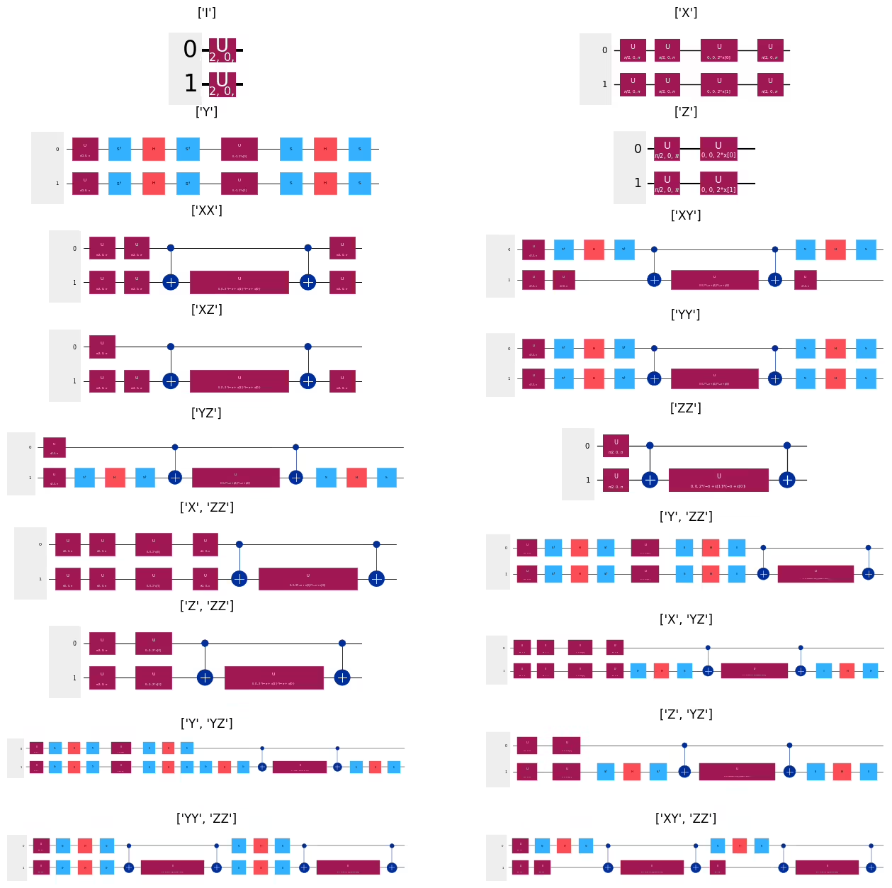
את האמור לעיל ניתן כמובן להרחיב כך שיכלול תמורות וחזרות נוספות של מטריצות פאולי. המשתתפים מוזמנים להתנסות עם האפשרויות האלו.

סקירה של מפות תכונות מובנות

ראית מספר שיטות לקידוד נתונים לתוך Circuit קוונטי:

• קידוד בסיסי
• קידוד אמפליטודה
• קידוד זווית
• קידוד פאזה
• קידוד צפוף

ראית כיצד לבנות מפות תכונות משלך בשיטות הקידוד האלו, וראית ארבע מפות תכונות מובנות שמנצלות קידוד זווית וקידוד פאזה:

• Efficient SU2
• מפת תכונות Z
• מפת תכונות ZZ
• מפת תכונות פאולי

מפות התכונות המובנות האלה נבדלו זו מזו במספר היבטים:

• העומק לכמות נתונה של תכונות מקודדות
• מספר ה-Qubits הנדרש לכמות נתונה של תכונות
• מידת ההסתבכות (שקשורה כמובן להבדלים האחרים)

הקוד שלהלן מחיל את ארבע מפות התכונות המובנות האלה על קידוד של קבוצת תכונות, ומציג את עומק ה-Circuit הדו-Qubit שמתקבל. מכיוון ששיעורי השגיאה של Gate דו-Qubit גבוהים בהרבה משיעורי שגיאה של Gate חד-Qubit, ייתכן שנהיה מעוניינים בעיקר בעומק של Gates דו-Qubit. בקוד שלהלן, אנחנו מקבלים ספירות של כל ה-Gates ב-Circuit על ידי פירוק ה-Circuit תחילה ואז שימוש ב-count_ops(), כפי שמוצג. כאן ה-Gates הדו-Qubit שמעניינים אותנו הם Gates מסוג 'cx':

# Initializing parameters and empty lists for depths
x = [0.1, 0.2]
n_data = []
zz2gates = []
su22gates = []
z2gates = []
p2gates = []

# Generating feature maps
for n in range(3, 10):
    x.append(n / 10)
    zzcircuit = zz_feature_map(n, reps=1, insert_barriers=True)
    zcircuit = z_feature_map(n, reps=1, insert_barriers=True)
    su2circuit = efficient_su2(n, reps=1, insert_barriers=True)
    pcircuit = pauli_feature_map(n, reps=1, paulis=["XX"], insert_barriers=True)
    # Getting the cx depths
    zzcx = zzcircuit.decompose().count_ops().get("cx")
    zcx = zcircuit.decompose().count_ops().get("cx")
    su2cx = su2circuit.decompose().count_ops().get("cx")
    pcx = pcircuit.decompose().count_ops().get("cx")

    # Appending the cx gate counts to the lists. We shift the zz and pauli data points, because they overlap.
    n_data.append(n)
    zz2gates.append(zzcx - 0.5)
    z2gates.append(0)
    su22gates.append(su2cx)
    p2gates.append(pcx + 0.5)

# Plot the output
plt.plot(n_data, p2gates, "bo")
plt.plot(n_data, zz2gates, "ro")
plt.plot(n_data, su22gates, "yo")
plt.plot(n_data, z2gates, "go")
plt.ylabel("CX Gates")
plt.xlabel("Data elements")
plt.legend(["Pauli", "ZZ", "SU2", "Z"])
# plt.suptitle('zz_feature_map(n)')
plt.show()

באופן כללי, מפות תכונות פאולי ו-ZZ יובילו לעומק Circuit גדול יותר ולמספר גבוה יותר של Gates דו-Qubit בהשוואה ל-efficient_su2 ולמפות תכונות Z.

מכיוון שמפות התכונות המובנות ב-Qiskit הן בעלות ישימות רחבה, לרוב לא נצטרך לעצב משלנו, במיוחד בשלב הלמידה. עם זאת, מומחים בלמידת מכונה קוונטית ככל הנראה יחזרו לנושא עיצוב מפות תכונות משלהם, כשהם מתמודדים עם שתי אתגרים מורכבים:

1. חומרה מודרנית: נוכחות הרעש והעלות הגבוהה של קוד תיקון שגיאות אומרים שיישומים עכשוויים יצטרכו לשקול דברים כמו יעילות חומרה ומזעור עומק Gate דו-Qubit.

2. מיפויים שמתאימים לבעיה הנדונה: זה דבר אחד לומר ש-zz_feature_map, למשל, קשה לסימולציה קלאסית ולכן מעניין. זה דבר אחר לגמרי ש-zz_feature_map יהיה מתאים באופן אידיאלי למשימת למידת המכונה שלך או לקבוצת הנתונים שלך. הביצועים של Circuits קוונטיים פרמטריים שונים על סוגים שונים של נתונים הם תחום פעיל של מחקר.

נסיים בהערה על יעילות חומרה.

מיפוי תכונות יעיל-חומרה

מיפוי תכונות יעיל-חומרה הוא מיפוי שמביא בחשבון מגבלות של מחשבים קוונטיים אמיתיים, מתוך מטרה לצמצם רעש ושגיאות בחישוב. כשמריצים Circuits קוונטיים על מחשבים קוונטיים קרובי-טווח, קיימות אסטרטגיות רבות לצמצום הרעש הטבוע בחומרה. אסטרטגיה מרכזית אחת ליעילות חומרה היא מזעור עומק ה-Circuit הקוונטי, כך שלרעש ולדקוהרנס יש פחות זמן לקלקל את החישוב. עומק Circuit קוונטי הוא מספר שלבי ה-Gate המסונכרנים בזמן הנדרשים לביצוע החישוב כולו (לאחר אופטימיזציית Circuit)[5]. זכור שעומק ה-Circuit ההגיוני המופשט עשוי להיות נמוך בהרבה מהעומק לאחר ש-Circuit עבר Transpilation למחשב קוונטי אמיתי.

Transpilation הוא התהליך של המרת ה-Circuit הקוונטי מהפשטה ברמה גבוהה לכזו שמוכנה לריצה על מחשב קוונטי אמיתי, תוך התחשבות במגבלות החומרה. למחשב קוונטי יש קבוצה מקורית של Gates חד-Qubit ודו-Qubit. המשמעות היא שכל Gates בקוד Qiskit צריכים לעבור Transpilation לקבוצת Gates החומרה המקוריים. למשל, ב-ibm_torino, QPU עם מעבד Heron r1 שהושלם ב-2023, ה-Gates המקוריים או ה-Basis Gates הם \{CZ, ID, RZ, SX, X\}. אלו הם Gate ה-controlled-Z הדו-Qubit, ו-Gates חד-Qubit שנקראים identity, $Z$-rotation, שורש ריבועי של NOT, ו-NOT, בהתאמה, ומספקים קבוצה אוניברסלית. כשמממשים Gates רב-Qubit כ-subcircuit שקול, נדרשים $CZ$ gates פיזיים דו-Qubit, יחד עם Gates חד-Qubit אחרים הזמינים בחומרה. בנוסף, כדי לבצע Gate דו-Qubit על זוג Qubits שאינם מחוברים פיזית, מוספים SWAP gates כדי להזיז מצבי Qubit בין Qubits לאפשר חיבור, מה שמוביל להארכה בלתי נמנעת של ה-Circuit. שימוש בארגומנט optimization שניתן להגדיר מ-0 עד לרמה הגבוהה ביותר של 3. לשליטה וגמישות רבה יותר, ניתן לנהל את pipeline של ה-Transpiler עם Qiskit Pass Manager. עיין ב-תיעוד Qiskit Transpiler למידע נוסף על Transpilation.

במחקר של Havlicek et al. 2019 [2], אחת הדרכים שבהן המחברים משיגים יעילות חומרה היא על ידי שימוש במפת תכונות $ZZ$ מכיוון שהיא התפשטות מסדר שני (ראה את הסעיף "מפת תכונות $ZZ$" לעיל). התפשטות מסדר $N$ כוללת Gates של $N$-Qubit. למחשבי IBM® הקוונטיים אין Gates מקוריים של $N$-Qubit, כאשר $N>2$, ולכן יישומם ידרוש פירוק ל-Gates CNOT דו-Qubit הזמינים בחומרה. דרך שנייה שבה המחברים ממזערים עומק היא על ידי בחירת טופולוגיית חיבור $ZZ$ שממפה ישירות לחיבורי הארכיטקטורה. אופטימיזציה נוספת שהם מבצעים היא כיוון לעבר subcircuit חומרה בעל ביצועים גבוהים ומחובר כראוי. דברים נוספים שכדאי לשקול הם מזעור מספר חזרות מפת התכונות ובחירת שיטת הסתבכות מותאמת אישית בעלת עומק נמוך או "ליניארית" במקום הסכמה "המלאה" שמסבכת את כל ה-Qubits.

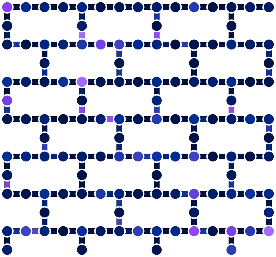
הגרפיקה לעיל מציגה רשת של צמתים וקשתות המייצגים Qubits פיזיים וחיבורי חומרה, בהתאמה. מפת החיבורים והביצועים של ibm_torino מוצגת עם כל Gates CZ הדו-Qubit האפשריים. ה-Qubits מקודדים בצבע על פני סקאלה המבוססת על זמן הרלקסציה T1 במיקרושניות (μs), כאשר זמני T1 ארוכים יותר טובים יותר ומוצגים בגוון בהיר יותר. קשתות החיבור מקודדות בצבע לפי שגיאת CZ, כאשר גוונים כהים יותר טובים יותר. מידע על מפרטי החומרה ניתן לגשת אליו בסכמת תצורת ה-Backend החומרה IBMQBackend.configuration().

מקורות

1. Maria Schuld and Francesco Petruccione, Supervised Learning with Quantum Computers, Springer 2018, doi:10.1007/978-3-319-96424-9.
2. Vojtech Havlicek et al., "Supervised Learning with Quantum Enhanced Feature Spaces." Nature, vol. 567 (2019): 209–212. https://arxiv.org/abs/1804.11326.
3. Ryan LaRose and Brian Coyle, "Robust data encodings for quantum classifiers", Physical Review A 102, 032420 (2020), doi:10.1103/PhysRevA.102.032420, arXiv:2003.01695.
4. Lou Grover and Terry Rudolph. "Creating Superpositions That Correspond to Efficiently Integrable Probability Distributions." arXiv:quant-ph/0208112, August 15, 2002, https://arxiv.org/abs/quant-ph/0208112.
5. Adrián Pérez-Salinas, Alba Cervera-Lierta, Elies Gil-Fuster, José I. Latorre, "Data re-uploading for a universal quantum classifier", Quantum 4, 226 (2020), ArXiv.org/abs/1907.02085.
6. Maria Schuld, Ryan Sweke, Johannes Jakob Meyer, "The effect of data encoding on the expressive power of variational quantum machine learning models", Phys. Rev. A 103, 032430 (2021), arxiv.org/abs/2008.08605

import qiskit

qiskit.version.get_version_info()