סימולציה של המילטוניאן Ising מוכה עם מעגלים דינמיים

הערכת שימוש: 7.5 דקות על מעבד Heron r3. (הערה: זוהי הערכה בלבד. זמן הריצה שלך עשוי להשתנות.) מעגלים דינמיים הם מעגלים עם feedforward קלאסי - במילים אחרות, הם מדידות באמצע המעגל ואחריהן פעולות לוגיקה קלאסית שקובעות פעולות קוונטיות המותנות בפלט הקלאסי. במדריך זה, אנו מדמים את מודל ה-Ising המוכה על סריג משושה של ספינים ומשתמשים במעגלים דינמיים כדי לממש אינטראקציות מעבר לקישוריות הפיזית של החומרה.

מודל ה-Ising נחקר באופן נרחב בתחומי הפיזיקה. הוא מדגם ספינים העוברים אינטראקציות Ising בין אתרי הסריג, כמו גם בעיטות מהשדה המגנטי המקומי בכל אתר. האבולוציה הזמנית המטרוטרת של הספינים שנבחנה במדריך זה, שנלקחה מ-[1], ניתנת על ידי היוניטרי הבא:

$$U(\theta)=\left(\prod_{\langle j, k\rangle} \exp \left(i \frac{\pi}{8} Z_j Z_k\right)\right)\left(\prod_j \exp \left(-i \frac{\theta}{2} X_j\right)\right)$$

כדי לבדוק את דינמיקת הספין, אנו חוקרים את המגנטיזציה הממוצעת של הספינים בכל אתר כפונקציה של צעדי Trotter. לכן, אנו בונים את ה-observable הבא:

$$\langle O\rangle = \frac{1}{N} \sum_i \langle Z_i \rangle$$

כדי לממש את האינטראקציה ZZ בין אתרי הסריג, אנו מציגים פתרון באמצעות תכונת המעגל הדינמי, המובילה לעומק two-qubit קצר משמעותית בהשוואה לשיטת הניתוב הסטנדרטית עם שערי SWAP. מצד שני, פעולות ה-feedforward הקלאסיות במעגלים דינמיים בדרך כלל יש להן זמני ביצוע ארוכים יותר משערים קוונטיים; לכן, למעגלים דינמיים יש מגבלות וטרייד-אופים. אנו גם מציגים דרך להוסיף רצף decoupling דינמי על קוביטים בהמתנה במהלך פעולת ה-feedforward הקלאסית באמצעות משך ה-stretch.

דרישות

לפני שמתחילים את המדריך, ודאו שהמוצרים הבאים מותקנים:

• Qiskit SDK v2.0 ומעלה עם תמיכה ב-visualization
• Qiskit Runtime v0.37 ומעלה עם תמיכה בויזואליזציה (pip install 'qiskit-ibm-runtime[visualization]')
• ספריית גרפים Rustworkx (pip install rustworkx)
• Qiskit Aer (pip install qiskit-aer)

הגדרה

# Added by doQumentation — required packages for this notebook
!pip install -q matplotlib numpy qiskit qiskit-aer qiskit-ibm-runtime rustworkx

import numpy as np
from typing import List
import rustworkx as rx
import matplotlib.pyplot as plt
from rustworkx.visualization import mpl_draw
from qiskit.circuit import (
    Parameter,
    QuantumCircuit,
    QuantumRegister,
    ClassicalRegister,
)
from qiskit.transpiler import CouplingMap
from qiskit.quantum_info import SparsePauliOp
from qiskit.circuit.classical import expr
from qiskit.transpiler.preset_passmanagers import (
    generate_preset_pass_manager,
)
from qiskit.transpiler import PassManager
from qiskit.circuit.library import RZGate, XGate
from qiskit.transpiler.passes import (
    ALAPScheduleAnalysis,
    PadDynamicalDecoupling,
)

from qiskit.transpiler.basepasses import TransformationPass
from qiskit.circuit.measure import Measure
from qiskit.transpiler.passes.utils.remove_final_measurements import (
    calc_final_ops,
)
from qiskit.circuit import Instruction

from qiskit.visualization import plot_circuit_layout
from qiskit.circuit.tools import pi_check

from qiskit_aer import AerSimulator
from qiskit_aer.primitives import SamplerV2 as Aer_Sampler

from qiskit_ibm_runtime import (
    QiskitRuntimeService,
    Batch,
    SamplerV2 as Sampler,
)
from qiskit_ibm_runtime.exceptions import QiskitBackendNotFoundError
from qiskit_ibm_runtime.visualization import (
    draw_circuit_schedule_timing,
)

שלב 1: מיפוי קלטים קלאסיים למעגל קוונטי

אנו מתחילים בהגדרת הסריג שיש לדמות. אנו בוחרים לעבוד עם סריג הדבש (נקרא גם משושה), שהוא גרף מישורי עם צמתים מדרגה 3. כאן, אנו מציינים את גודל הסריג, את פרמטרי המעגל הרלוונטיים המעניינים בדינמיקה המטרוטרת. אנו מדמים את האבולוציה הזמנית המטרוטרת תחת מודל ה-Ising תחת שלושה ערכי $\theta$ שונים של השדה המגנטי המקומי.

hex_rows = 3  # specify lattice size
hex_cols = 5
depths = range(9)  # specify Trotter steps
zz_angle = np.pi / 8  # parameter for ZZ interaction
max_angle = np.pi / 2  # max theta angle
points = 3  # number of theta parameters

θ = Parameter("θ")
params = np.linspace(0, max_angle, points)

def make_hex_lattice(hex_rows=1, hex_cols=1):
    """Define hexagon lattice."""
    hex_cmap = CouplingMap.from_hexagonal_lattice(
        hex_rows, hex_cols, bidirectional=False
    )
    data = list(hex_cmap.physical_qubits)
    graph = hex_cmap.graph.to_undirected(multigraph=False)
    edge_colors = rx.graph_misra_gries_edge_color(graph)
    layer_edges = {color: [] for color in edge_colors.values()}
    for edge_index, color in edge_colors.items():
        layer_edges[color].append(graph.edge_list()[edge_index])
    return data, layer_edges, hex_cmap, graph

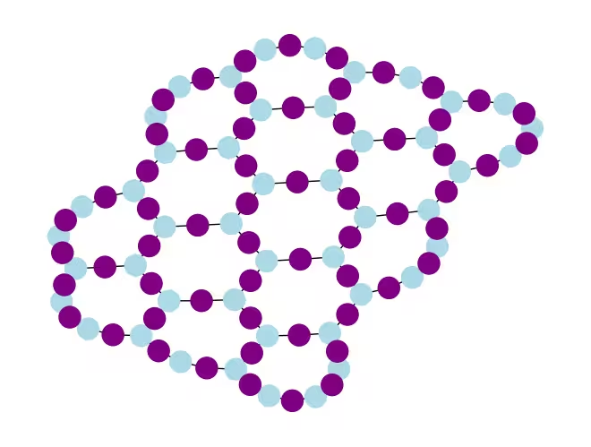
בואו נתחיל בדוגמת בדיקה קטנה:

hex_rows_test = 1
hex_cols_test = 2

data_test, layer_edges_test, hex_cmap_test, graph_test = make_hex_lattice(
    hex_rows=hex_rows_test, hex_cols=hex_cols_test
)

# display a small example for illustration
node_colors_test = ["lightblue"] * len(graph_test.node_indices())
pos = rx.graph_spring_layout(
    graph_test,
    k=5 / np.sqrt(len(graph_test.nodes())),
    repulsive_exponent=1,
    num_iter=150,
)
mpl_draw(graph_test, node_color=node_colors_test, pos=pos)

נשתמש בדוגמה הקטנה להמחשה ולסימולציה. למטה אנו גם בונים דוגמה גדולה כדי להראות שניתן להרחיב את זרימת העבודה לגדלים גדולים.

data, layer_edges, hex_cmap, graph = make_hex_lattice(
    hex_rows=hex_rows, hex_cols=hex_cols
)
num_qubits = len(data)
print(f"num_qubits = {num_qubits}")

# display the honeycomb lattice to simulate
node_colors = ["lightblue"] * len(graph.node_indices())
pos = rx.graph_spring_layout(
    graph,
    k=5 / np.sqrt(num_qubits),
    repulsive_exponent=1,
    num_iter=150,
)
mpl_draw(graph, node_color=node_colors, pos=pos)
plt.show()

num_qubits = 46

בניית מעגלים יוניטריים

עם גודל הבעיה והפרמטרים שצוינו, אנו עכשיו מוכנים לבנות את המעגל המפורמט שמדמה את האבולוציה הזמנית המטרוטרת של $U(\theta)$ עם צעדי Trotter שונים, שצוינו על ידי ארגומנט ה-depth. למעגל שאנו בונים יש שכבות מתחלפות של שערי Rx($\theta$) ושערי Rzz. שערי ה-Rzz ממשים את האינטראקציות ZZ בין ספינים מזווגים, שיוצבו בין כל אתר סריג שצוין על ידי ארגומנט ה-layer_edges.

def gen_hex_unitary(
    num_qubits=6,
    zz_angle=np.pi / 8,
    layer_edges=[
        [(0, 1), (2, 3), (4, 5)],
        [(1, 2), (3, 4), (5, 0)],
    ],
    θ=Parameter("θ"),
    depth=1,
    measure=False,
    final_rot=True,
):
    """Build unitary circuit."""
    circuit = QuantumCircuit(num_qubits)
    # Build trotter layers
    for _ in range(depth):
        for i in range(num_qubits):
            circuit.rx(θ, i)
        circuit.barrier()
        for coloring in layer_edges.keys():
            for e in layer_edges[coloring]:
                circuit.rzz(zz_angle, e[0], e[1])
        circuit.barrier()
    # Optional final rotation, set True to be consistent with Ref. [1]
    if final_rot:
        for i in range(num_qubits):
            circuit.rx(θ, i)
    if measure:
        circuit.measure_all()

    return circuit

הצגת מעגל הבדיקה הקטן:

circ_unitary_test = gen_hex_unitary(
    num_qubits=len(data_test),
    layer_edges=layer_edges_test,
    θ=Parameter("θ"),
    depth=1,
    measure=True,
)
circ_unitary_test.draw(output="mpl", fold=-1)

באופן דומה, בנייה של המעגלים היוניטריים של הדוגמה הגדולה בצעדי Trotter שונים וה-observable להערכת ערך התוחלת.

circuits_unitary = []
for depth in depths:
    circ = gen_hex_unitary(
        num_qubits=num_qubits,
        layer_edges=layer_edges,
        θ=Parameter("θ"),
        depth=depth,
        measure=True,
    )
    circuits_unitary.append(circ)

observables_unitary = SparsePauliOp.from_sparse_list(
    [("Z", [i], 1 / num_qubits) for i in range(num_qubits)],
    num_qubits=num_qubits,
)

בניית מימוש מעגל דינמי

חלק זה מדגים את המימוש העיקרי של המעגל הדינמי לדמות את אותה אבולוציה זמנית מטרוטרת. שימו לב שסריג הדבש שאנו רוצים לדמות אינו תואם לסריג הכבד של קוביטי החומרה. דרך ישירה אחת למפות את המעגל לחומרה היא להציג סדרה של פעולות SWAP כדי להביא קוביטים מתקשרים זה ליד זה, כדי לממש את האינטראקציה ZZ. כאן אנו מדגישים גישה חלופית באמצעות מעגלים דינמיים כפתרון, שמדגימה שאנחנו יכולים להשתמש בשילוב של חישוב קוונטי וקלאסי בזמן אמת בתוך מעגל ב-Qiskit כדי לממש אינטראקציות מעבר לשכנים הקרובים ביותר.

במימוש המעגל הדינמי, האינטראקציה ZZ מיושמת ביעילות על ידי שימוש בקוביטי עזר, מדידה באמצע המעגל, ו-feedforward. כדי להבין זאת, שימו לב שסיבובי ZZ מיישמים גורם פאזה $e^{i\theta}$ למצב על בסיס הזוגיות שלו. לשני קוביטים, מצבי הבסיס החישוביים הם $|00\rangle$, $|01\rangle$, $|10\rangle$, ו-$|11\rangle$. שער סיבוב ZZ מיישם גורם פאזה למצבים $|01\rangle$ ו-$|10\rangle$ שהזוגיות שלהם (מספר האחדים במצב) היא אי-זוגית ומשאיר מצבים זוגיים ללא שינוי. להלן מתואר כיצד נוכל לממש ביעילות אינטראקציות ZZ על שני קוביטים באמצעות מעגלים דינמיים.

1. חישוב זוגיות לקוביט עזר: במקום ליישם ישירות ZZ על שני קוביטים, אנו מציגים קוביט שלישי, קוביט העזר, כדי לאחסן את מידע הזוגיות של שני קוביטי הנתונים. אנו משלבים את העזר עם כל קוביט נתונים באמצעות שערי CX מקוביט הנתונים לקוביט העזר.

2. יישום סיבוב Z של קוביט יחיד לקוביט העזר: זה משום שלעזר יש את מידע הזוגיות של שני קוביטי הנתונים, מה שמיישם ביעילות את סיבוב ZZ על קוביטי הנתונים.

3. מדידת קוביט העזר בבסיס X: זהו השלב המפתח שמקריס את מצב קוביט העזר, ותוצאת המדידה אומרת לנו מה קרה:

   • מדידה 0: כאשר נצפית תוצאה 0, למעשה יישמנו סיבוב $ZZ(\theta)$ נכון לקוביטי הנתונים שלנו.

   • מדידה 1: כאשר נצפית תוצאה 1, יישמנו $ZZ(\theta + \pi)$ במקום זאת.

4. יישום שער תיקון כאשר מודדים 1: אם מדדנו 1, אנו מיישמים שערי Z לקוביטי הנתונים כדי "לתקן" את הפאזה הנוספת $\pi$.

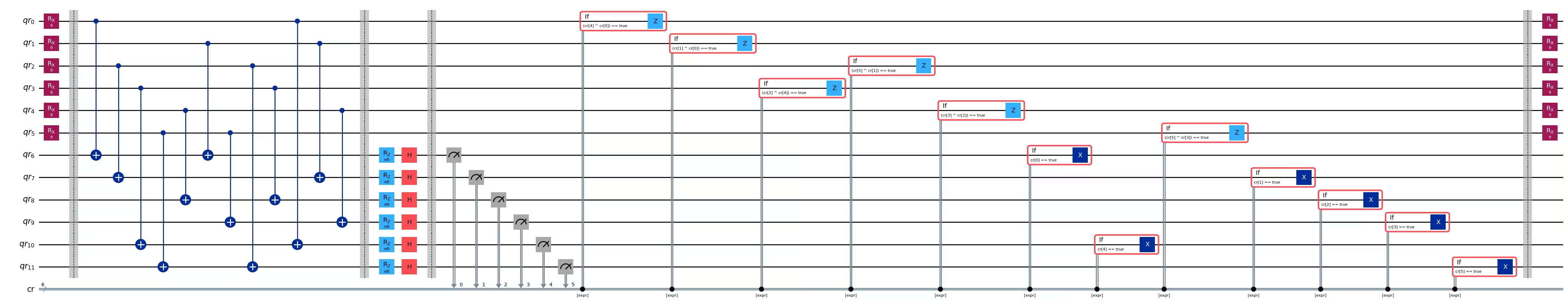
המעגל המתקבל הוא הבא:

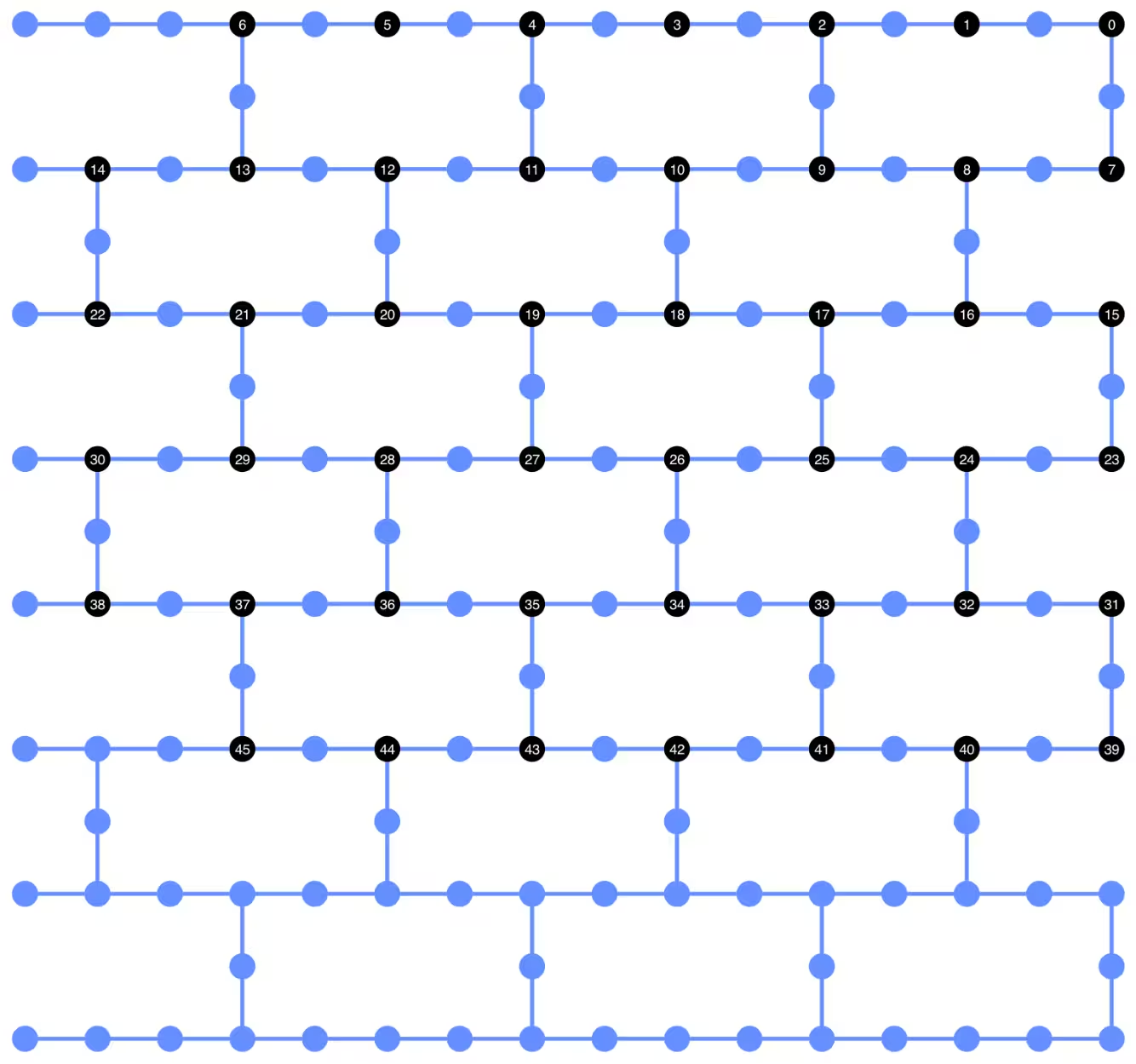
כאשר אנו מאמצים גישה זו כדי לדמות סריג דבש, המעגל המתקבל משתלב בצורה מושלמת בחומרה עם סריג heavy-hex: כל קוביטי הנתונים נמצאים באתרים מדרגה-3 של הסריג, היוצרים סריג משושה. כל זוג של קוביטי נתונים משתף קוביט עזר השוכן באתר מדרגה-2. למטה, אנו בונים את סריג הקוביטים למימוש המעגל הדינמי, מציגים קוביטי עזר (מוצגים במעגלים הסגולים הכהים יותר).

def make_lattice(hex_rows=1, hex_cols=1):
    """Define heavy-hex lattice and corresponding lists of data and ancilla nodes."""
    hex_cmap = CouplingMap.from_hexagonal_lattice(
        hex_rows, hex_cols, bidirectional=False
    )
    data = list(hex_cmap.physical_qubits)

    heavyhex_cmap = CouplingMap()
    for d in data:
        heavyhex_cmap.add_physical_qubit(d)

    # make coupling map
    a = len(data)
    for edge in hex_cmap.get_edges():
        heavyhex_cmap.add_physical_qubit(a)
        heavyhex_cmap.add_edge(edge[0], a)
        heavyhex_cmap.add_edge(edge[1], a)
        a += 1
    ancilla = list(range(len(data), a))
    qubits = data + ancilla

    # color edges
    graph = heavyhex_cmap.graph.to_undirected(multigraph=False)
    edge_colors = rx.graph_misra_gries_edge_color(graph)
    layer_edges = {color: [] for color in edge_colors.values()}
    for edge_index, color in edge_colors.items():
        layer_edges[color].append(graph.edge_list()[edge_index])

    # construct observable
    obs_hex = SparsePauliOp.from_sparse_list(
        [("Z", [i], 1 / len(data)) for i in data],
        num_qubits=len(qubits),
    )

    return (data, qubits, ancilla, layer_edges, heavyhex_cmap, graph, obs_hex)

הצגת סריג ה-heavy-hex עבור קוביטי נתונים וקוביטי עזר בקנה מידה קטן:

(data, qubits, ancilla, layer_edges, heavyhex_cmap, graph, obs_hex) = (
    make_lattice(hex_rows=hex_rows, hex_cols=hex_cols)
)

print(f"number of data qubits = {len(data)}")
print(f"number of ancilla qubits = {len(ancilla)}")

node_colors = []
for node in graph.node_indices():
    if node in ancilla:
        node_colors.append("purple")
    else:
        node_colors.append("lightblue")

pos = rx.graph_spring_layout(
    graph,
    k=1 / np.sqrt(len(qubits)),
    repulsive_exponent=2,
    num_iter=200,
)

# Visualize the graph, blue circles are data qubits and purple circles are ancillas
mpl_draw(graph, node_color=node_colors, pos=pos)
plt.show()

number of data qubits = 46
number of ancilla qubits = 60

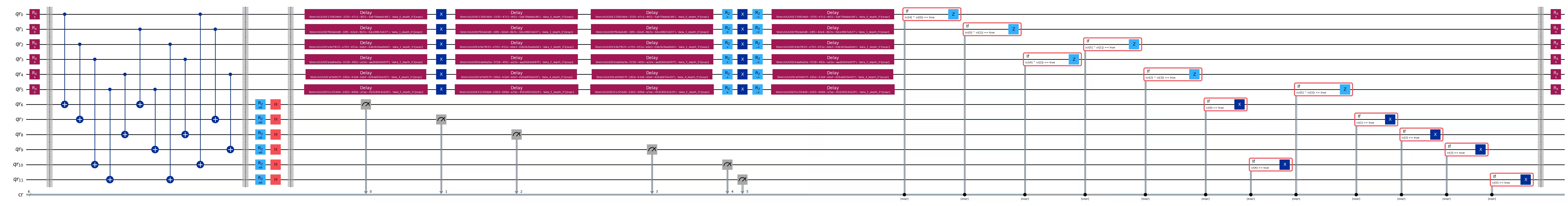
למטה, אנו בונים את המעגל הדינמי לאבולוציה הזמנית המטרוטרת. שערי ה-RZZ מוחלפים במימוש המעגל הדינמי באמצעות השלבים שתוארו לעיל.

def gen_hex_dynamic(
    depth=1,
    zz_angle=np.pi / 8,
    θ=Parameter("θ"),
    hex_rows=1,
    hex_cols=1,
    measure=False,
    add_dd=True,
):
    """Build dynamic circuits."""
    (data, qubits, ancilla, layer_edges, heavyhex_cmap, graph, obs_hex) = (
        make_lattice(hex_rows=hex_rows, hex_cols=hex_cols)
    )
    # Initialize circuit
    qr = QuantumRegister(len(qubits), "qr")
    cr = ClassicalRegister(len(ancilla), "cr")
    circuit = QuantumCircuit(qr, cr)

    for k in range(depth):
        # Single-qubit Rx layer
        for d in data:
            circuit.rx(θ, d)
        circuit.barrier()

        # CX gates from data qubits to ancilla qubits
        for same_color_edges in layer_edges.values():
            for e in same_color_edges:
                circuit.cx(e[0], e[1])
        circuit.barrier()

        # Apply Rz rotation on ancilla qubits and rotate into X basis
        for a in ancilla:
            circuit.rz(zz_angle, a)
            circuit.h(a)
        # Add barrier to align terminal measurement
        circuit.barrier()

        # Measure ancilla qubits
        for i, a in enumerate(ancilla):
            circuit.measure(a, i)
        d2ros = {}
        a2ro = {}
        # Retrieve ancilla measurement outcomes
        for a in ancilla:
            a2ro[a] = cr[ancilla.index(a)]

        # For each data qubit, retrieve measurement outcomes of neighboring ancilla qubits
        for d in data:
            ros = [a2ro[a] for a in heavyhex_cmap.neighbors(d)]
            d2ros[d] = ros

        # Build classical feedforward operations (optionally add DD on idling data qubits)
        for d in data:
            if add_dd:
                circuit = add_stretch_dd(circuit, d, f"data_{d}_depth_{k}")

            # # XOR the neighboring readouts of the data qubit; if True, apply Z to it
            ros = d2ros[d]
            parity = ros[0]
            for ro in ros[1:]:
                parity = expr.bit_xor(parity, ro)
            with circuit.if_test(expr.equal(parity, True)):
                circuit.z(d)

        # Reset the ancilla if its readout is 1
        for a in ancilla:
            with circuit.if_test(expr.equal(a2ro[a], True)):
                circuit.x(a)
        circuit.barrier()

    # Final single-qubit Rx layer to match the unitary circuits
    for d in data:
        circuit.rx(θ, d)

    if measure:
        circuit.measure_all()
    return circuit, obs_hex

def add_stretch_dd(qc, q, name):
    """Add XpXm DD sequence."""
    s = qc.add_stretch(name)
    qc.delay(s, q)
    qc.x(q)
    qc.delay(s, q)
    qc.delay(s, q)
    qc.rz(np.pi, q)
    qc.x(q)
    qc.rz(-np.pi, q)
    qc.delay(s, q)
    return qc

Dynamical decoupling (DD) ותמיכה במשך stretch

אזהרה אחת של שימוש במימוש המעגל הדינמי כדי לממש את האינטראקציה ZZ היא שהמדידה באמצע המעגל ופעולות ה-feedforward הקלאסיות בדרך כלל לוקחות זמן ארוך יותר לביצוע משערים קוונטיים. כדי לדכא דה-קוהרנטיות של קוביט במהלך זמן ההמתנה לפעולות הקלאסיות להתרחש, הוספנו רצף dynamical decoupling (DD) לאחר פעולת המדידה על קוביטי העזר, ולפני פעולת Z המותנית על קוביט הנתונים, לפני הצהרת ה-if_test.

רצף ה-DD מתווסף על ידי הפונקציה add_stretch_dd(), שמשתמשת ב-משכי stretch כדי לקבוע את מרווחי הזמן בין שערי ה-DD. משך stretch הוא דרך לציין משך זמן מתיחה עבור פעולת ה-delay כך שמשך העיכוב יכול לגדול כדי למלא את זמן ההמתנה של הקוביט. משתני המשך שצוינו על ידי stretch נפתרים בזמן הקומפילציה למשכים רצויים שמספקים אילוץ מסוים. זה מאוד שימושי כאשר התזמון של רצפי DD חיוני להשגת ביצועי דיכוי שגיאות טובים. לפרטים נוספים על סוג ה-stretch, ראה את תיעוד ה-OpenQASM. כרגע, התמיכה בסוג stretch ב-Qiskit Runtime היא ניסיונית. לפרטים על מגבלות השימוש שלו, אנא עיינו ב-סעיף המגבלות של תיעוד ה-stretch.

באמצעות הפונקציות שהוגדרו לעיל, אנו בונים את מעגלי האבולוציה הזמנית המטרוטרים, עם ובלי DD, ואת ה-observables המתאימים. אנו מתחילים בהצגת המעגל הדינמי של דוגמה קטנה:

hex_rows_test = 1
hex_cols_test = 1

(
    data_test,
    qubits_test,
    ancilla_test,
    layer_edges_test,
    heavyhex_cmap_test,
    graph_test,
    obs_hex_test,
) = make_lattice(hex_rows=hex_rows_test, hex_cols=hex_cols_test)

node_colors = []
for node in graph_test.node_indices():
    if node in ancilla_test:
        node_colors.append("purple")
    else:
        node_colors.append("lightblue")
pos = rx.graph_spring_layout(
    graph_test,
    k=5 / np.sqrt(len(qubits_test)),
    repulsive_exponent=2,
    num_iter=150,
)

# display a small example for illustration
node_colors_test = ["lightblue"] * len(graph_test.node_indices())
mpl_draw(graph_test, node_color=node_colors, pos=pos)

circuit_dynamic_test, obs_dynamic_test = gen_hex_dynamic(
    depth=1,
    θ=Parameter("θ"),
    hex_rows=hex_rows_test,
    hex_cols=hex_cols_test,
    measure=False,
    add_dd=False,
)
circuit_dynamic_test.draw("mpl", fold=-1)

circuit_dynamic_dd_test, _ = gen_hex_dynamic(
    depth=1,
    θ=Parameter("θ"),
    hex_rows=hex_rows_test,
    hex_cols=hex_cols_test,
    measure=False,
    add_dd=True,
)
circuit_dynamic_dd_test.draw("mpl", fold=-1)

באופן דומה, בניית המעגלים הדינמיים לדוגמה הגדולה:

circuits_dynamic = []
circuits_dynamic_dd = []
observables_dynamic = []
for depth in depths:
    circuit, obs = gen_hex_dynamic(
        depth=depth,
        θ=Parameter("θ"),
        hex_rows=hex_rows,
        hex_cols=hex_cols,
        measure=True,
        add_dd=False,
    )
    circuits_dynamic.append(circuit)

    circuit_dd, _ = gen_hex_dynamic(
        depth=depth,
        θ=Parameter("θ"),
        hex_rows=hex_rows,
        hex_cols=hex_cols,
        measure=True,
        add_dd=True,
    )
    circuits_dynamic_dd.append(circuit_dd)
    observables_dynamic.append(obs)

שלב 2: אופטימיזציה של הבעיה לביצוע על חומרה

אנו עכשיו מוכנים לטרנספייל את המעגל לחומרה. נטרנספייל גם את המימוש הסטנדרטי היוניטרי וגם את מימוש המעגל הדינמי לחומרה.

כדי לטרנספייל לחומרה, אנו תחילה משתמשים ב-backend. אם זמין, נבחר backend שבו הוראת ה-MidCircuitMeasure (measure_2) נתמכת.

service = QiskitRuntimeService()
try:
    backend = service.least_busy(
        operational=True,
        simulator=False,
        use_fractional_gates=True,
        filters=lambda b: "measure_2" in b.supported_instructions,
    )
except QiskitBackendNotFoundError:
    backend = service.least_busy(
        operational=True,
        simulator=False,
        use_fractional_gates=True,
    )

Transpilation למעגלים דינמיים

ראשית, אנו מטרנספיילים את המעגלים הדינמיים, עם ובלי הוספת רצף ה-DD. כדי להבטיח שאנו משתמשים באותו סט של קוביטים פיזיים בכל המעגלים לתוצאות עקביות יותר, אנו תחילה מטרנספיילים את המעגל פעם אחת, ולאחר מכן משתמשים ב-layout שלו לכל המעגלים הבאים, שצוין על ידי initial_layout ב-pass manager. לאחר מכן אנו בונים את ה-primitive unified blocs (PUBs) כקלט פרימיטיבי Sampler.

pm_temp = generate_preset_pass_manager(
    optimization_level=3,
    backend=backend,
)
isa_temp = pm_temp.run(circuits_dynamic[-1])
dynamic_layout = isa_temp.layout.initial_index_layout(filter_ancillas=True)

pm = generate_preset_pass_manager(
    optimization_level=3, backend=backend, initial_layout=dynamic_layout
)

dynamic_isa_circuits = [pm.run(circ) for circ in circuits_dynamic]
dynamic_pubs = [(circ, params) for circ in dynamic_isa_circuits]

dynamic_isa_circuits_dd = [pm.run(circ) for circ in circuits_dynamic_dd]
dynamic_pubs_dd = [(circ, params) for circ in dynamic_isa_circuits_dd]

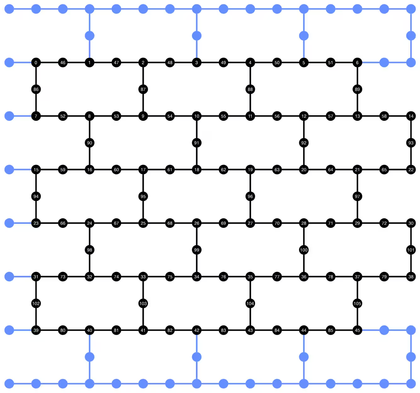
אנו יכולים להציג את פריסת הקוביטים של המעגל המטרנספייל למטה. המעגלים השחורים מציגים את קוביטי הנתונים וקוביטי העזר המשמשים במימוש המעגל הדינמי.

def _heron_coords_r2():
    cord_map = np.array(
        [
            [
                0,
                1,
                2,
                3,
                4,
                5,
                6,
                7,
                8,
                9,
                10,
                11,
                12,
                13,
                14,
                15,
                3,
                7,
                11,
                15,
                0,
                1,
                2,
                3,
                4,
                5,
                6,
                7,
                8,
                9,
                10,
                11,
                12,
                13,
                14,
                15,
                1,
                5,
                9,
                13,
                0,
                1,
                2,
                3,
                4,
                5,
                6,
                7,
                8,
                9,
                10,
                11,
                12,
                13,
                14,
                15,
                3,
                7,
                11,
                15,
                0,
                1,
                2,
                3,
                4,
                5,
                6,
                7,
                8,
                9,
                10,
                11,
                12,
                13,
                14,
                15,
                1,
                5,
                9,
                13,
                0,
                1,
                2,
                3,
                4,
                5,
                6,
                7,
                8,
                9,
                10,
                11,
                12,
                13,
                14,
                15,
                3,
                7,
                11,
                15,
                0,
                1,
                2,
                3,
                4,
                5,
                6,
                7,
                8,
                9,
                10,
                11,
                12,
                13,
                14,
                15,
                1,
                5,
                9,
                13,
                0,
                1,
                2,
                3,
                4,
                5,
                6,
                7,
                8,
                9,
                10,
                11,
                12,
                13,
                14,
                15,
                3,
                7,
                11,
                15,
                0,
                1,
                2,
                3,
                4,
                5,
                6,
                7,
                8,
                9,
                10,
                11,
                12,
                13,
                14,
                15,
            ],
            -1
            * np.array([j for i in range(15) for j in [i] * [16, 4][i % 2]]),
        ],
        dtype=int,
    )

    hcords = []
    ycords = cord_map[0]
    xcords = cord_map[1]
    for i in range(156):
        hcords.append([xcords[i] + 1, np.abs(ycords[i]) + 1])

    return hcords

plot_circuit_layout(
    dynamic_isa_circuits_dd[8],
    backend,
    qubit_coordinates=_heron_coords_r2(),
    view="virtual",
)

הערה

אם אתם מקבלים שגיאות לגבי neato לא נמצא מ-plot_circuit_layout(), ודאו שחבילת graphviz מותקנת וזמינה ב-PATH שלכם. אם היא מתקנת למיקום לא ברירת מחדל (לדוגמה, שימוש ב-homebrew ב-MacOS), ייתכן שתצטרכו לעדכן את משתנה הסביבה PATH שלכם. ניתן לעשות זאת בתוך מחברת זו באמצעות הדברים הבאים:

import os
os.environ['PATH'] = f"path/to/neato{os.pathsep}{os.environ['PATH']}"

dynamic_isa_circuits[1].draw(fold=-1, output="mpl", idle_wires=False)

dynamic_isa_circuits_dd[1].draw(fold=-1, output="mpl", idle_wires=False)

Transpile באמצעות MidCircuitMeasure

MidCircuitMeasure היא תוספת לפעולות המדידה הזמינות, מכוילת במיוחד לביצוע מדידות באמצע המעגל. הוראת MidCircuitMeasure ממופה להוראת measure_2 הנתמכת על ידי ה-backends. שימו לב ש-measure_2 לא נתמכת בכל ה-backends. אתם יכולים להשתמש ב-service.backends(filters=lambda b: "measure_2" in b.supported_instructions) כדי למצוא backends שתומכים בזה. כאן, אנו מראים כיצד לטרנספייל את המעגל כך שהמדידות באמצע המעגל שהוגדרו במעגל מבוצעות באמצעות פעולת MidCircuitMeasure, אם ה-backend תומך בזה.

למטה, אנו מדפיסים את המשך להוראת measure_2 והוראת measure הסטנדרטית.

print(
    f'Mid-circuit measurement `measure_2` duration: {backend.instruction_durations.get('measure_2',0) * backend.dt * 1e9/1e3} μs'
)
print(
    f'Terminal measurement `measure` duration: {backend.instruction_durations.get('measure',0) * backend.dt *1e9/1e3} μs'
)

Mid-circuit measurement `measure_2` duration:  1.624 μs
Terminal measurement `measure` duration: 2.2 μs

"""Pass that replaces terminal measures in the middle of the circuit with
MidCircuitMeasure instructions."""

class ConvertToMidCircuitMeasure(TransformationPass):
    """This pass replaces terminal measures in the middle of the circuit with
    MidCircuitMeasure instructions.
    """

    def __init__(self, target):
        super().__init__()
        self.target = target

    def run(self, dag):
        """Run the pass on a dag."""
        mid_circ_measure = None
        for inst in self.target.instructions:
            if isinstance(inst[0], Instruction) and inst[0].name.startswith(
                "measure_"
            ):
                mid_circ_measure = inst[0]
                break
        if not mid_circ_measure:
            return dag

        final_measure_nodes = calc_final_ops(dag, {"measure"})
        for node in dag.op_nodes(Measure):
            if node not in final_measure_nodes:
                dag.substitute_node(node, mid_circ_measure, inplace=True)

        return dag

pm = PassManager(ConvertToMidCircuitMeasure(backend.target))

dynamic_isa_circuits_meas2 = [pm.run(circ) for circ in dynamic_isa_circuits]
dynamic_pubs_meas2 = [(circ, params) for circ in dynamic_isa_circuits_meas2]

dynamic_isa_circuits_dd_meas2 = [
    pm.run(circ) for circ in dynamic_isa_circuits_dd
]
dynamic_pubs_dd_meas2 = [
    (circ, params) for circ in dynamic_isa_circuits_dd_meas2
]

Transpilation למעגלים יוניטריים

כדי ליצור השוואה הוגנת בין המעגלים הדינמיים והמקבילה היוניטרית שלהם, אנו משתמשים באותו סט של קוביטים פיזיים המשמשים במעגלים הדינמיים עבור קוביטי הנתונים כ-layout לטרנספיילינג של המעגלים היוניטריים.

init_layout = [
    dynamic_layout[ind] for ind in range(circuits_unitary[0].num_qubits)
]

pm = generate_preset_pass_manager(
    target=backend.target,
    initial_layout=init_layout,
    optimization_level=3,
)

def transpile_minimize(circ: QuantumCircuit, pm: PassManager, iterations=10):
    """Transpile circuits for specified number of iterations and return the one with smallest two-qubit gate depth"""
    circs = [pm.run(circ) for i in range(iterations)]
    circs_sorted = sorted(
        circs,
        key=lambda x: x.depth(lambda x: x.operation.num_qubits == 2),
    )
    return circs_sorted[0]

unitary_isa_circuits = []
for circ in circuits_unitary:
    circ_t = transpile_minimize(circ, pm, iterations=100)
    unitary_isa_circuits.append(circ_t)

unitary_pubs = [(circ, params) for circ in unitary_isa_circuits]

אנו מציגים את פריסת הקוביטים של המעגלים היוניטריים המטרנספיילים. המעגלים השחורים מציינים את הקוביטים הפיזיים המשמשים לטרנספיילינג של המעגלים היוניטריים והאינדקסים שלהם מתאימים לאינדקסים של הקוביטים הווירטואליים. על ידי השוואת זה עם ה-layout שהוצג עבור המעגלים הדינמיים, אנו יכולים לאשר שהמעגלים היוניטריים משתמשים באותו סט של קוביטים פיזיים כמו קוביטי הנתונים במעגלים הדינמיים.

plot_circuit_layout(
    unitary_isa_circuits[-1],
    backend,
    qubit_coordinates=_heron_coords_r2(),
    view="virtual",
)

אנו עכשיו מוסיפים את רצף ה-DD למעגלים המטרנספיילים ובונים את ה-PUBs המתאימים להגשת עבודות.

pm_dd = PassManager(
    [
        ALAPScheduleAnalysis(target=backend.target),
        PadDynamicalDecoupling(
            dd_sequence=[
                XGate(),
                RZGate(np.pi),
                XGate(),
                RZGate(-np.pi),
            ],
            spacing=[1 / 4, 1 / 2, 0, 0, 1 / 4],
            target=backend.target,
        ),
    ]
)

unitary_isa_circuits_dd = pm_dd.run(unitary_isa_circuits)
unitary_pubs_dd = [(circ, params) for circ in unitary_isa_circuits_dd]

השוואת עומק שער two-qubit של מעגלים יוניטריים ודינמיים

# compare circuit depth of unitary and dynamic circuit implementations
unitary_depth = [
    unitary_isa_circuits[i].depth(lambda x: x.operation.num_qubits == 2)
    for i in range(len(unitary_isa_circuits))
]

dynamic_depth = [
    dynamic_isa_circuits[i].depth(lambda x: x.operation.num_qubits == 2)
    for i in range(len(dynamic_isa_circuits))
]

plt.plot(
    list(range(len(unitary_depth))),
    unitary_depth,
    label="unitary circuits",
    color="#be95ff",
)
plt.plot(
    list(range(len(dynamic_depth))),
    dynamic_depth,
    label="dynamic circuits",
    color="#ff7eb6",
)
plt.xlabel("Trotter steps")
plt.ylabel("Two-qubit depth")
plt.legend()

<matplotlib.legend.Legend at 0x374225760>

היתרון העיקרי של המעגל מבוסס המדידה הוא שכאשר מיישמים אינטראקציות ZZ מרובות, שכבות ה-CX יכולות להיות מקבילות, והמדידות יכולות להתרחש בו זמנית. זה משום שכל האינטראקציות ZZ מתחלפות, כך שניתן לבצע את החישוב עם עומק מדידה 1. לאחר טרנספיילינג המעגלים, אנו מבחינים שהגישה של המעגל הדינמי מניבה עומק two-qubit קצר משמעותית מהגישה היוניטרית הסטנדרטית, עם האזהרה שהמדידה הנוספת באמצע המעגל וה-feedforward הקלאסי עצמם לוקחים זמן ומציגים מקורות שגיאה משלהם.

שלב 3: ביצוע באמצעות פרימיטיבים של Qiskit

מצב בדיקה מקומי

לפני הגשת העבודות לחומרה, אנו יכולים להריץ סימולציה קטנה של המעגל הדינמי באמצעות מצב הבדיקה המקומי.

aer_sim = AerSimulator()
pm = generate_preset_pass_manager(backend=aer_sim, optimization_level=1)
circuit_dynamic_test.measure_all()
isa_qc = pm.run(circuit_dynamic_test)
with Batch(backend=aer_sim) as batch:
    sampler = Sampler(mode=batch)
    result = sampler.run([(isa_qc, params)]).result()

print(
    "Simulated average magnetization at trotter step = 1 at three theta values"
)
result[0].data["meas"].expectation_values(obs_dynamic_test[0])

Simulated average magnetization at trotter step = 1 at three theta values

array([ 0.16666667,  0.01855469, -0.13476562])

סימולציית MPS

למעגלים גדולים, אנו יכולים להשתמש בסימולטור matrix_product_state (MPS), שמספק תוצאה משוערת לערך התוחלת לפי ממד הקשר שנבחר. אנו משתמשים מאוחר יותר בתוצאות סימולציית MPS כקו הבסיס להשוואת התוצאות מהחומרה.

# The MPS simulation below took approximately 7 minutes to run on a laptop with Apple M1 chip

mps_backend = AerSimulator(
    method="matrix_product_state",
    matrix_product_state_truncation_threshold=1e-5,
    matrix_product_state_max_bond_dimension=100,
)
mps_sampler = Aer_Sampler.from_backend(mps_backend)

shots = 4096

data_sim = []
for j in range(points):
    circ_list = [
        circ.assign_parameters([params[j]]) for circ in circuits_unitary
    ]

    mps_job = mps_sampler.run(circ_list, shots=shots)
    result = mps_job.result()

    point_data = [
        result[d].data["meas"].expectation_values(observables_unitary)
        for d in depths
    ]

    data_sim.append(point_data)  # data at one theta value

data_sim = np.array(data_sim)

עם המעגלים וה-observables מוכנים, אנו עכשיו מבצעים אותם על החומרה באמצעות פרימיטיבי Sampler.

כאן אנו מגישים שלוש עבודות עבור unitary_pubs, dynamic_pubs, ו-dynamic_pubs_dd. כל אחת היא רשימה של מעגלים מפורמטים המתאימים לתשעה צעדי Trotter שונים עם שלושה פרמטרי $\theta$ שונים.

shots = 10000

with Batch(backend=backend) as batch:
    sampler = Sampler(mode=batch)

    sampler.options.experimental = {
        "execution": {
            "scheduler_timing": True
        },  # set to True to retrieve circuit timing info
    }

    job_unitary = sampler.run(unitary_pubs, shots=shots)
    print(f"unitary: {job_unitary.job_id()}")

    job_unitary_dd = sampler.run(unitary_pubs_dd, shots=shots)
    print(f"unitary_dd: {job_unitary_dd.job_id()}")

    job_dynamic = sampler.run(dynamic_pubs, shots=shots)
    print(f"dynamic: {job_dynamic.job_id()}")

    job_dynamic_dd = sampler.run(dynamic_pubs_dd, shots=shots)
    print(f"dynamic_dd: {job_dynamic_dd.job_id()}")

    job_dynamic_meas2 = sampler.run(dynamic_pubs_meas2, shots=shots)
    print(f"dynamic_meas2: {job_dynamic_meas2.job_id()}")

    job_dynamic_dd_meas2 = sampler.run(dynamic_pubs_dd_meas2, shots=shots)
    print(f"dynamic_dd_meas2: {job_dynamic_dd_meas2.job_id()}")

unitary: d5dtt0ldq8ts73fvbhj0
unitary: d5dtt11smlfc739onuag
dynamic: d5dtt1hsmlfc739onuc0
dynamic_dd: d5dtt25jngic73avdne0
dynamic_meas2: d5dtt2ldq8ts73fvbhm0
dynamic_dd_meas2: d5dtt2tjngic73avdnf0

שלב 4: עיבוד לאחר החזרת תוצאות בפורמט קלאסי רצוי

לאחר שהעבודות הושלמו, אנו יכולים לשלוף את משך המעגל ממטא-נתוני תוצאות העבודה ולהציג את מידע לוח הזמנים של המעגל. לקריאה נוספת על הצגת מידע התזמון של מעגל, עיינו ב-דף זה.

# Circuit durations is reported in the unit of `dt` which can be retrieved from `Backend` object
unitary_durations = [
    job_unitary.result()[i].metadata["compilation"]["scheduler_timing"][
        "circuit_duration"
    ]
    for i in depths
]

dynamic_durations = [
    job_dynamic.result()[i].metadata["compilation"]["scheduler_timing"][
        "circuit_duration"
    ]
    for i in depths
]

dynamic_durations_meas2 = [
    job_dynamic_meas2.result()[i].metadata["compilation"]["scheduler_timing"][
        "circuit_duration"
    ]
    for i in depths
]

result_dd = job_dynamic_dd.result()[1]
circuit_schedule_dd = result_dd.metadata["compilation"]["scheduler_timing"][
    "timing"
]

# to visualize the circuit schedule, one can show the figure below
fig_dd = draw_circuit_schedule_timing(
    circuit_schedule=circuit_schedule_dd,
    included_channels=None,
    filter_readout_channels=False,
    filter_barriers=False,
    width=1000,
)

# Save to a file since the figure is large
fig_dd.write_html("scheduler_timing_dd.html")

אנו משרטטים את משכי המעגל עבור מעגלים יוניטריים והמעגלים הדינמיים. מהגרף למטה, אנו יכולים לראות שלמרות הזמן הנדרש למדידות באמצע המעגל ופעולות קלאסיות, מימוש המעגל הדינמי עם measure_2 מביא למשכי מעגל דומים למימוש היוניטרי.

# visualize circuit durations

def convert_dt_to_microseconds(circ_duration: List, backend_dt: float):
    dt = backend_dt * 1e6  # dt in microseconds
    return list(map(lambda x: x * dt, circ_duration))

dt = backend.target.dt
plt.plot(
    depths,
    convert_dt_to_microseconds(unitary_durations, dt),
    color="#be95ff",
    linestyle=":",
    label="unitary",
)
plt.plot(
    depths,
    convert_dt_to_microseconds(dynamic_durations, dt),
    color="#ff7eb6",
    linestyle="-.",
    label="dynamic",
)
plt.plot(
    depths,
    convert_dt_to_microseconds(dynamic_durations_meas2, dt),
    color="#ff7eb6",
    linestyle="-.",
    marker="s",
    mfc="none",
    label="dynamic w/ meas2",
)

plt.xlabel("Trotter steps")
plt.ylabel(r"Circuit durations in $\mu$s")
plt.legend()

<matplotlib.legend.Legend at 0x17f73c6e0>

לאחר שהעבודות הושלמו, אנו שולפים את הנתונים למטה ומחשבים את המגנטיזציה הממוצעת שהוערכה על ידי ה-observables observables_unitary או observables_dynamic שבנינו קודם לכן.

runs = {
    "unitary": (
        job_unitary,
        [observables_unitary] * len(circuits_unitary),
    ),
    "unitary_dd": (
        job_unitary_dd,
        [observables_unitary] * len(circuits_unitary),
    ),
    # Omitting Dyn w/o DD and Dynamic w/ DD plots for better readability
    # "dynamic": (job_dynamic, observables_dynamic),
    # "dynamic_dd": (job_dynamic_dd, observables_dynamic),
    "dynamic_meas2": (job_dynamic_meas2, observables_dynamic),
    "dynamic_dd_meas2": (
        job_dynamic_dd_meas2,
        observables_dynamic,
    ),
}

data_dict = {}
for key, (job, obs) in runs.items():
    data = []
    for i in range(points):
        data.append(
            [
                job.result()[ind].data["meas"].expectation_values(obs[ind])[i]
                for ind in depths
            ]
        )
    data_dict[key] = data

למטה אנו משרטטים את מגנטיזציית הספין כפונקציה של צעדי Trotter בערכי $\theta$ שונים, המתאימים לעוצמות שונות של השדה המגנטי המקומי. אנו משרטטים גם את תוצאות סימולציית MPS המחושבות מראש עבור המעגלים היוניטריים האידיאליים, יחד עם התוצאות הניסיוניות מהבאות:

1. הפעלת המעגלים היוניטריים עם DD
2. הפעלת המעגלים הדינמיים עם DD ו-MidCircuitMeasure

plt.figure(figsize=(10, 6))

colors = ["#0f62fe", "#be95ff", "#ff7eb6"]
for i in range(points):
    plt.plot(
        depths,
        data_sim[i],
        color=colors[i],
        linestyle="solid",
        label=f"θ={pi_check(i*max_angle/(points-1))} (MPS)",
    )
    # plt.plot(
    #     depths,
    #     data_dict["unitary"][i],
    #     color=colors[i],
    #     linestyle=":",
    #     label=f"θ={pi_check(i*max_angle/(points-1))} (Unitary)",
    # )

    plt.plot(
        depths,
        data_dict["unitary_dd"][i],
        color=colors[i],
        marker="o",
        mfc="none",
        linestyle=":",
        label=f"θ={pi_check(i*max_angle/(points-1))} (Unitary w/DD)",
    )

    # Omitting Dyn w/o DD and Dynamic w/ DD plots for better readability
    # plt.plot(
    #     depths,
    #     data_dict["dynamic"][i],
    #     color=colors[i],
    #     linestyle="-.",
    #     label=f"θ={pi_check(i*max_angle/(points-1))} (Dyn w/o DD)",
    # )
    # plt.plot(
    #     depths,
    #     data_dict["dynamic_dd"][i],
    #     marker="D",
    #     mfc="none",
    #     color=colors[i],
    #     linestyle="-.",
    #     label=f"θ={pi_check(i*max_angle/(points-1))} (Dynamic w/ DD)",
    # )

    # plt.plot(
    #     depths,
    #     data_dict["dynamic_meas2"][i],
    #     color=colors[i],
    #     marker="s",
    #     mfc="none",
    #     linestyle=':',
    #     label=f"θ={pi_check(i*max_angle/(points-1))} (Dynamic w/ MidCircuitMeas)",
    # )

    plt.plot(
        depths,
        data_dict["dynamic_dd_meas2"][i],
        color=colors[i],
        marker="*",
        markersize=8,
        linestyle=":",
        label=f"θ={pi_check(i*max_angle/(points-1))} (Dynamic w/ DD & MidCircuitMeas)",
    )

plt.xlabel("Trotter steps", fontsize=16)
plt.ylabel("Average magnetization", fontsize=16)
plt.xticks(rotation=45)
handles, labels = plt.gca().get_legend_handles_labels()
plt.legend(
    handles,
    labels,
    loc="upper right",
    bbox_to_anchor=(1.46, 1.0),
    shadow=True,
    ncol=1,
)
plt.title(
    f"{hex_rows}x{hex_cols} hex ring, {num_qubits} data qubits, {len(ancilla)} ancilla qubits \n{backend.name}: Sampler"
)
plt.show()

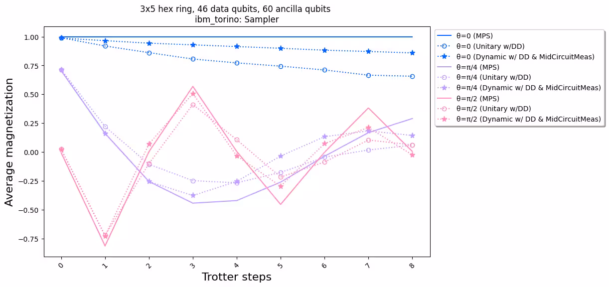
כאשר אנו משווים את התוצאות הניסיוניות עם הסימולציה, אנו רואים שמימוש המעגל הדינמי (קו מקווקו עם כוכבים) בסך הכל יש לו ביצועים טובים יותר מהמימוש היוניטרי הסטנדרטי (קו מקווקו עם עיגולים). לסיכום, אנו מציגים מעגלים דינמיים כפתרון לסימולציה של מודלי ספין Ising על סריג דבש, טופולוגיה שאינה מקורית לחומרה. פתרון המעגל הדינמי מאפשר אינטראקציות ZZ בין קוביטים שאינם שכנים הקרובים ביותר, עם עומק שער two-qubit קצר יותר משימוש בשערי SWAP, במחיר הצגת קוביטי עזר נוספים ופעולות feedforward קלאסיות.

הפניות

[1] Quantum computing with Qiskit, by Javadi-Abhari, A., Treinish, M., Krsulich, K., Wood, C.J., Lishman, J., Gacon, J., Martiel, S., Nation, P.D., Bishop, L.S., Cross, A.W. and Johnson, B.R., 2024. arXiv preprint arXiv:2405.08810 (2024)