תצפית על דינמיקת הדרונים לא-אבליים חסינה וקוהרנטית במעבדי קוונטים רועשים
הערכת שימוש: 6 דקות על מעבד Heron (ibm_boston או שווה ערך) (הערה: זו הערכה בלבד. זמן הריצה שלכם עשוי להשתנות.)
תוצרי למידה
-
איך תיאוריות כיול-סריג לא-אבליות (ספציפית SU(2)) ניתנות לניסוח מחדש באמצעות מסגרת ה-Loop-String-Hadron (LSH) לסימולציה קוונטית יעילה
-
איך לבנות מעגלי אבולוציית זמן מטרוטרזים (Trotterized) עבור המילטוניאן קירוב של תורת כיול SU(2) ולמפות אותם על קיוביטים
-
איך להריץ מעגלים אלה על חומרת IBM Quantum® באמצעות הפרימיטיב Estimator של Qiskit עם הקלת שגיאות קריאה
דרישות מוקדמות
-
היכרות בסיסית עם מושגי תורת השדות הקוונטית (מועיל אך לא נדרש; סעיף הרקע מכסה את היסודות)
רקע
מוטיבציה
כרומודינמיקה קוונטית (QCD), תורת הכיול SU(3) של הכוח החזק, קושרת קווארקים להדרונים ושולטת בכליאה ובשבירת מיתרים. שיטות QCD סריג קלאסיות מצטיינות בתכונות סטטיות אך אינן יכולות לסמלץ דינמיקה בזמן-אמת בשל בעיית הסימן. מחשבים קוונטיים מציעים דרך עוקפת מכשול זה על ידי קידוד דרגות חופש של שדה הכיול ישירות על קיוביטים.
מדריך זה מדגים סימולציה כזו: שימוש בחומרת IBM Quantum לסימולציית התפשטות הדרונים בזמן-אמת בתורת כיול-סריג SU(2) דו-ממדית (1+1) — תורת הכיול הלא-אבלית הפשוטה ביותר ואבן דרך לעבר QCD מלאה.
ההמילטוניאן של Kogut-Susskind
התיאוריה מנוסחת על סריג מרחבי חד-ממדי עם פרמיונים מדורגים (חומר) באתרים ושדות כיול SU(2) על קישורים. לאחר שינוי קנה מידה לצורה חסרת ממד, ההמילטוניאן הוא:
כאשר הוא אנרגיית השדה הכרומואלקטרי, הוא איבר המסה המדורגת, הוא איבר האינטראקציה חומר-כיול (קפיצה), מקודד את מסת הפרמיון, ו- הוא עוצמת האינטראקציה. הגבול הרציף של התיאוריה נמצא ב- וב-.
מסגרת ה-Loop-String-Hadron (LSH)
אתגר מרכזי הוא שמרחב הילברט של שדה הכיול בכל קישור הוא אינסופי-ממדי. מסגרת Loop-String-Hadron (LSH) מטפלת בכך על ידי ניסוח מחדש של התיאוריה במונחים של משתנים אינווריאנטיים לכיול — לולאות של שטף, מיתרים המחברים מטענים מופרדים, והדרונים (זוגות פרמיונים שהם סינגלט כיול באתר). בבסיס LSH, חוק גאוס מתקיים באופן אוטומטי מעצם הבנייה, כך שכל מצב בסיס הוא פיזיקלי. כל אתר סריג מאופיין בשלושה מספרים קוונטיים המייצגים את מספר הלולאה, המיתר הנכנס, והמיתר היוצא, כאשר הם פרמיוניים ו- הוא בוזוני. מספר הפרמיון המקומי מוגדר מאלה כ- עבור אתרים זוגיים ו- עבור אתרים אי-זוגיים.
מהמילטוניאן מלא למעגל הקוונטי: שלוש קירובים מרכזיים
המעגל הקוונטי לא מסמלץ את ההמילטוניאן המלא של SU(2) במדויק. במקום זאת, הוא מיישם סדרה מבוקרת של קירובים התקפים במשטר הצימוד-החלש (). הבנת מה כן ומה לא מקורב היא חיונית:
קירוב 1 — גבול צימוד-חלש עבור : ההמילטוניאן המלא של האינטראקציה (משוואה 16 ב-[1]) מכיל מקדמים שתלויים במספר הקוונטי הבוזוני דרך איברים כמו . במשטר הצימוד-החלש (), הדינמיקה נשלטת על ידי האיבר החשמלי , שמעדיף מצבים עם גדול. עבור , היחס וכל המקדמים האלה מצטמצמים ליחידה. ההמילטוניאן של האינטראקציה מצטמצם אז לקפיצה מקומית טהורה בין שכנים קרובים:
שהוא בלתי-תלוי ב- ופועל רק על הקיוביטים הפרמיוניים .
קירוב 2 — שטף-ממוצע-גלובלי עבור : האנרגיה החשמלית תלויה ב- בכל קישור. בוואקום של הצימוד-החלש, גדול ואחיד בקירוב. מחליפים את ערכי התלויים-באתר בממוצע גלובלי בודד , מה שהופך את לפאזה אלכסונית פרופורציונלית לתצורת הפרמיון בכל אתר:
כאשר מסכם על פני אתרים בתצורה הפרמיונית , ו- הוא פאזה גלובלית שניתן להתעלם ממנה.
קירוב 3 — Trotterization: אופרטור אבולוציית הזמן עבור צעד באורך מתפרק כך:
כאשר , , ו-. פירוק Trotter מסדר ראשון זה מכניס שגיאה שמתאפסת כאשר . אנחנו קובעים לאורך כל הדרך.
התוצאה של שלושת הקירובים האלה היא ששני הקיוביטים הפרמיוניים בלבד לכל אתר הם דינמיים — דרגת החופש הבוזונית נספגה לתוך פרמטרים אפקטיביים. זה נותן מעגל קומפקטי עם קיוביטים עבור אתרי סריג, כאשר לכל צעד Trotter יש עומק שערים דו-קיוביטיים קבוע (13 לצעד).
מה מדריך זה מסמלץ
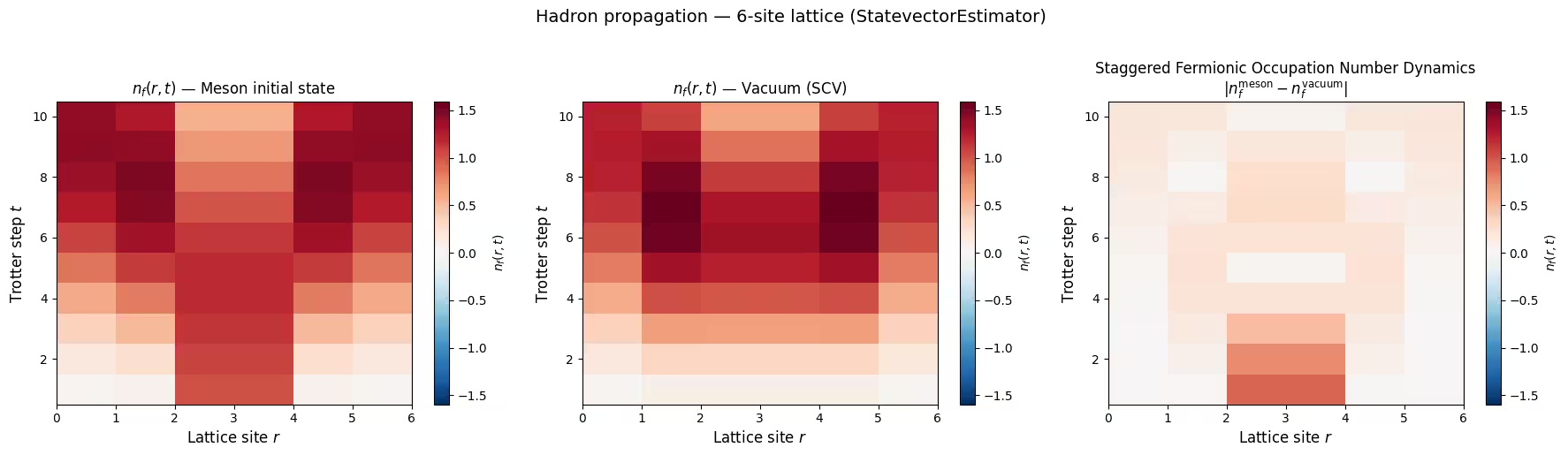
המדריך מסמלץ התפשטות הדרונים: החל מוואקום הצימוד-החזק (מצב מכפלה), מציבים מזון (meson) במרכז הסריג ומתפתחים בזמן. פרוטוקול המדידה הדיפרנציאלית — הרצת המעגל עם ובלי המזון המרכזי, ולאחר מכן חיסור — מבודד את אות ההדרון הקוהרנטי הן מרעש חומרה והן מאפקטי גבול. התוצאה היא דפוס חרוט-אור של תנודות צפיפות פרמיונים האופייני למצב נשימה של מזון כלוא.
דרישות
לפני תחילת מדריך זה, התקינו את הבאים:
-
ערכת הפיתוח Qiskit SDK v2.0 ומעלה, עם תמיכת ויזואליזציה
-
Qiskit Runtime v0.22 ומעלה (
pip install qiskit-ibm-runtime) -
חבילת Pauli Propagation (
pip install pauli-prop) -
NumPy (
pip install numpy) -
Matplotlib (
pip install matplotlib)
הגדרה
התחילו בייבוא הספריות הדרושות והגדרת פונקציות העזר שבונות את המעגלים הקוונטיים עבור אבולוציית הזמן של LSH. יש שלוש פונקציות ליבה לבניית מעגלים:
-
pair_hamiltonian_circuit: מיישמת את היוניטרי הדו-קיוביטי עבור המילטוניאן האינטראקציה המקורב בין אתרים שכנים. פירוק השערים הוא: . -
electric_hamiltonian_circuit: מיישמת את היוניטרי הדו-קיוביטי עבור אנרגיית שדה חשמלי מקורבת בכל אתר. פירוק השערים הוא: . -
construct_circuit: מרכיבה את המעגל המלא בעל Trotterization, מסדרת בשכבות איברי אינטראקציה, חשמל, ומסה עם שערי SWAP כדי לנהל קישוריות קיוביטים.
# Added by doQumentation — required packages for this notebook
!pip install -q matplotlib numpy pauli-prop qiskit qiskit-ibm-runtime
# Import libraries

import numpy as np
import matplotlib.pyplot as plt
from matplotlib.colors import TwoSlopeNorm
from qiskit.circuit import QuantumCircuit
from qiskit.quantum_info import SparsePauliOp
from typing import Optional

import warnings

warnings.filterwarnings("ignore")
def pair_hamiltonian_circuit(c: float) -> QuantumCircuit:
    """Two-qubit unitary for the approximate interaction Hamiltonian H_I.

    Implements exp(-i * c * H_I^approx) for one pair of neighboring sites,
    where c = delta_tau * x.
    """
    qc_temp = QuantumCircuit(2)
    qc_temp.cx(1, 0)
    qc_temp.h(1)
    qc_temp.rz(-c, 1)
    qc_temp.cx(0, 1)
    qc_temp.rz(c, 1)
    qc_temp.cx(0, 1)
    qc_temp.h(1)
    qc_temp.cx(1, 0)
    return qc_temp

def electric_hamiltonian_circuit(theta: float) -> QuantumCircuit:
    """Two-qubit unitary for the approximate electric field Hamiltonian H_E.

    Implements exp(-i * theta * H_E^approx) for one lattice site,
    where theta = -delta_tau * (n_bar_l / 2 + 3/4).
    """
    qc_temp = QuantumCircuit(2)
    qc_temp.x(0)
    qc_temp.rz(theta / 2, 0)
    qc_temp.cx(0, 1)
    qc_temp.rz(-theta / 2, 1)
    qc_temp.cx(0, 1)
    qc_temp.rz(theta / 2, 1)
    qc_temp.x(0)
    return qc_temp

def construct_circuit(
    num_lattice_point: int,
    num_trotter_steps: int,
    c: float,
    theta: float,
    m: float,
    theory: Optional[int] = 2,
    barriers: Optional[bool] = False,
    measurement: Optional[bool] = False,
    add_init_state: Optional[bool] = True,
    inverse_mid: Optional[bool] = False,
) -> QuantumCircuit:
    """Construct the full Trotterized time-evolution circuit.

    Builds a circuit implementing n Trotter steps of the approximate SU(2)
    LSH Hamiltonian evolution. The qubit layout uses a zigzag ordering:
    n_i(0), n_i(1), n_o(0), n_o(1), n_i(2), n_i(3), n_o(2), n_o(3), ...
    which minimizes the number of SWAP layers needed.

    Args:
        num_lattice_point: Number of lattice sites
        (num_qubits = 2 * num_lattice_point).
        num_trotter_steps: Number of Trotter steps.
        c: Interaction parameter (delta_tau * x).
        theta: Electric field phase parameter.
        m: Mass parameter (m_tilde = delta_tau * mu).
        theory: 1 for single chain, 2 for SU(2). Default 2.
        barriers: Insert barriers between Trotter layers for
        visualization.
        measurement: Append measurements at the end.
        add_init_state: Prepare the half-filled (strong-coupling vacuum)
        initial state.
        inverse_mid: Swap the central sites
        (for differential measurement protocol).
    """
    num_qubits = theory * num_lattice_point
    qc = QuantumCircuit(num_qubits)

    if num_trotter_steps <= 0:
        return qc

    # --- Initial state preparation ---
    if add_init_state:
        i = 1
        while i < num_lattice_point:
            for j in range(theory):
                qc.x(i + j * num_lattice_point)
            i = i + 2
        if inverse_mid:
            mid_lattice_qubits = [num_qubits // 2 - 1, num_qubits // 2]
            qc.x(mid_lattice_qubits)
    else:
        i = 1
        while i < num_qubits - 1:
            qc.swap(i, i + 1)
            i = i + 4

    # --- Trotter steps ---
    for step in range(num_trotter_steps):
        if barriers:
            qc.barrier()

        # First SWAP layer (skipped at step 0 — absorbed into initial state mapping)
        if step > 0:
            i = 1
            while i < num_qubits - 1:
                qc.swap(i, i + 1)
                i = i + 4

        # First layer of pair interactions
        j = 0
        while j < num_qubits - 2:
            circ = pair_hamiltonian_circuit(c)
            qc.compose(circ, [j, j + 1], inplace=True)
            j = j + 2
        if num_lattice_point % 2 == 0:
            circ = pair_hamiltonian_circuit(c)
            qc.compose(circ, [j, j + 1], inplace=True)

        # Second SWAP layer
        i = 1
        while i < num_qubits - 1:
            qc.swap(i, i + 1)
            i = i + theory

        # Second layer of pair interactions
        j = 2
        while j < num_qubits - 3:
            circ = pair_hamiltonian_circuit(c)
            qc.compose(circ, [j, j + 1], inplace=True)
            j = j + 2
        if num_lattice_point % 2 != 0:
            circ = pair_hamiltonian_circuit(c)
            qc.compose(circ, [j, j + 1], inplace=True)

        # Third SWAP layer
        i = 3
        while i < num_qubits - 1:
            qc.swap(i, i + 1)
            i = i + 2 * theory

        # Electric field term
        if theta != 0:
            e_circ = electric_hamiltonian_circuit(theta)
            for j in range(num_lattice_point):
                qc.compose(e_circ, [2 * j, 2 * j + 1], inplace=True)

        # Mass term: Rz(-m_tilde) for even sites, Rz(m_tilde) for odd sites
        for q in range(num_qubits):
            if q % 2 == 0:
                qc.rz(-1 * m, q)
            else:
                qc.rz(m, q)

    if measurement:
        qc.measure_all()

    return qc
def get_probabilities(expval: float):
    """Convert a Z-expectation value to site occupation probability.

    Since <Z> = p(0) - p(1), the occupation probability is p(1) = (1 - <Z>) / 2.
    """
    p1 = round((1 - expval) / 2, 3)
    return p1

def get_number(expval_data, num_lattice_point):
    """Convert raw Z-expectation values to staggered fermion number n_f at each site.

    n_f(r) = n_i(r) + n_o(r)           for even r
    n_f(r) = 2 - [n_i(r) + n_o(r)]     for odd r

    The two qubits per site encode (n_i, n_o), and occupation probabilities
    give us <n_i> and <n_o>.
    """
    N = []
    for expvals in expval_data:
        Pstep = [get_probabilities(expval) for expval in expvals]
        Nstep = []
        for k in range(num_lattice_point):
            val = Pstep[2 * k] + Pstep[2 * k + 1]
            a = 2 * (k % 2) + (1 - 2 * (k % 2)) * val
            Nstep.append(float(a))
        N.append(Nstep)
    return N

def calculate_difference(N, N_mid, num_lattice_point):
    """Differential measurement protocol: |n_f(meson) - n_f(vacuum)|.

    Subtracting the vacuum (SCV) evolution from the meson evolution
    isolates the coherent hadron signal from symmetric noise and boundary effects.
    """
    N_diff = []
    for i in range(len(N)):
        Nstep_diff = []
        for j in range(num_lattice_point):
            Nstep_diff.append(abs(N[i][j] - N_mid[i][j]))
        N_diff.append(Nstep_diff)
    return N_diff
דוגמת סימולטור בקנה מידה קטן
תחילה, הדגימו את זרימת העבודה בקנה מידה קטן באמצעות סריג בן שישה אתרים (12 קיוביטים), כך שתוכלו לאמת את בניית המעגל ולהבין את התצפיות הפיזיקליות לפני ההרצה על חומרה.
שלב 1: מיפוי קלטים קלאסיים לבעיה קוונטית
הגדירו את הפרמטרים הפיזיקליים התואמים למשטר הצימוד-החלש שנחקר במאמר (, ). הפרמטרים הנגזרים של המעגל הם:
-
(פרמטר אינטראקציה)
-
(פאזת שדה חשמלי)
-
(פרמטר מסה)
עבור כל מספר צעדי Trotter, בנו שני מעגלים: אחד המאתחל מזון במרכז (inverse_mid=True) ואחד המכין את וואקום הצימוד-החזק (inverse_mid=False). פרוטוקול המדידה הדיפרנציאלית מחסר את האבולוציה של הוואקום כדי לבודד את אות ההדרון.
# Physical / circuit parameters
num_lattice_point = 6  # 6 lattice sites -> 12 qubits for SU(2)
num_qubits = 2 * num_lattice_point
c = 0.15  # delta_tau * x
theta = 0.01  # electric field phase
m = 0.03  # m_tilde = delta_tau * mu
trotter_steps = range(1, 11)  # 10 Trotter steps

print(f"Lattice sites: {num_lattice_point}, Qubits: {num_qubits}")
print(f"Parameters: c={c}, theta={theta}, m_tilde={m}")
Lattice sites: 6, Qubits: 12
Parameters: c=0.15, theta=0.01, m_tilde=0.03
# Build circuits: meson initial state and vacuum (SCV) initial state
circuits_mid = [
    construct_circuit(
        num_lattice_point,
        d,
        c,
        theta,
        m,
        barriers=False,
        measurement=False,
        add_init_state=True,
        inverse_mid=True,
    )
    for d in trotter_steps
]

circuits = [
    construct_circuit(
        num_lattice_point,
        d,
        c,
        theta,
        m,
        barriers=False,
        measurement=False,
        add_init_state=True,
        inverse_mid=False,
    )
    for d in trotter_steps
]

# Visualize a single Trotter step
print(
    f"Circuit for 1 Trotter step: {circuits[0].num_qubits} qubits, depth {circuits[0].depth()}"
)
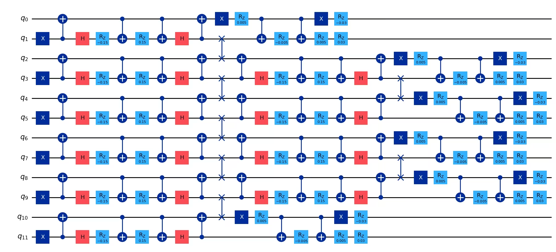
circuits[0].draw("mpl", fold=-1)
Circuit for 1 Trotter step: 12 qubits, depth 26
שלב 2: אופטימיזציה של הבעיה להרצה על חומרה קוונטית
הגדירו את התצפיות: מדידות חד-קיוביטיות על כל קיוביט. מ- ניתן לחלץ הסתברויות תפוסה ולאחר מכן את מספר הפרמיון המדורג בכל אתר סריג .
# Z observable on each qubit
observables = [
    SparsePauliOp("I" * i + "Z" + "I" * (num_qubits - i - 1))
    for i in range(num_qubits)
]

print(f"Number of observables: {len(observables)}")
Number of observables: 12
שלב 3: הרצה באמצעות הפרימיטיבים של Qiskit
השתמשו ב-StatevectorEstimator לסימולציה מדויקת חסרת רעש בקנה מידה קטן.
from qiskit.primitives import StatevectorEstimator

estimator = StatevectorEstimator()

# Run meson circuits
pubs_mid = [(circuit, observables) for circuit in circuits_mid]
result_mid = estimator.run(pubs_mid).result()

# Run vacuum (SCV) circuits
pubs = [(circuit, observables) for circuit in circuits]
result = estimator.run(pubs).result()

# Extract expectation values
raw_expvals_mid = [
    result_mid[i].data.evs[::-1] for i in range(len(circuits_mid))
]
raw_expvals = [result[i].data.evs[::-1] for i in range(len(circuits))]

print(f"Computed expectation values for {len(raw_expvals)} Trotter steps")
Computed expectation values for 10 Trotter steps
שלב 4: עיבוד לאחר ריצה והחזרת התוצאה בפורמט קלאסי רצוי
המירו ערכי תוחלת למספר הפרמיון המדורג והפעילו את פרוטוקול המדידה הדיפרנציאלית (מזון וואקום) כדי להפיק את מפת החום של התפשטות ההדרון. זה משחזר את המבנה של איור 3 מהמאמר המקורי: אתר סריג בציר ה-x, צעד Trotter (זמן) בציר ה-y, ו- כסולם הצבע.
# Compute fermion numbers
N_mid_sim = get_number(raw_expvals_mid, num_lattice_point)
N_sim = get_number(raw_expvals, num_lattice_point)
N_diff_sim = calculate_difference(N_mid_sim, N_sim, num_lattice_point)

# --- Reproduce Figure 3 style: Staggered Fermionic Occupation Number Dynamics ---
fig, axes = plt.subplots(1, 3, figsize=(18, 5))

# Convert to numpy arrays for plotting
N_mid_arr = np.array(N_mid_sim)
N_arr = np.array(N_sim)
N_diff_arr = np.array(N_diff_sim)

# Color scheme
vmax = max(max(sublist) for sublist in N_arr)
vmin = -vmax

# Meson evolution
norm1 = TwoSlopeNorm(vmin=vmin, vcenter=0, vmax=vmax)
im0 = axes[0].imshow(
    N_mid_arr,
    aspect="auto",
    origin="lower",
    cmap="RdBu_r",
    norm=norm1,
    extent=[0, num_lattice_point, 0.5, len(trotter_steps) + 0.5],
)
axes[0].set_xlabel("Lattice site $r$", fontsize=12)
axes[0].set_ylabel("Trotter step $t$", fontsize=12)
axes[0].set_title("$n_f(r,t)$ — Meson initial state", fontsize=12)
plt.colorbar(im0, ax=axes[0], label="$n_f(r,t)$")

# Vacuum (SCV) evolution
im1 = axes[1].imshow(
    N_arr,
    aspect="auto",
    origin="lower",
    cmap="RdBu_r",
    norm=norm1,
    extent=[0, num_lattice_point, 0.5, len(trotter_steps) + 0.5],
)
axes[1].set_xlabel("Lattice site $r$", fontsize=12)
axes[1].set_ylabel("Trotter step $t$", fontsize=12)
axes[1].set_title("$n_f(r,t)$ — Vacuum (SCV)", fontsize=12)
plt.colorbar(im1, ax=axes[1], label="$n_f(r,t)$")

# Differential: meson - vacuum
norm2 = TwoSlopeNorm(vmin=vmin, vcenter=0, vmax=vmax)
im2 = axes[2].imshow(
    N_diff_arr,
    aspect="auto",
    origin="lower",
    cmap="RdBu_r",
    norm=norm2,
    extent=[0, num_lattice_point, 0.5, len(trotter_steps) + 0.5],
)
axes[2].set_xlabel("Lattice site $r$", fontsize=12)
axes[2].set_ylabel("Trotter step $t$", fontsize=12)
axes[2].set_title(
    "Staggered Fermionic Occupation Number Dynamics\n$|n_f^{\\mathrm{meson}} - n_f^{\\mathrm{vacuum}}|$",
    fontsize=12,
)
plt.colorbar(im2, ax=axes[2], label="$n_f(r,t)$")

plt.suptitle(
    f"Hadron propagation — {num_lattice_point}-site lattice (StatevectorEstimator)",
    fontsize=14,
    y=1.02,
)
plt.tight_layout()
plt.show()
דוגמת חומרה בקנה מידה גדול
עכשיו אנחנו מרחיבים לסריג בן 30 אתרים (60 קיוביטים) על חומרת IBM Quantum. בקנה מידה זה, המעגל ב-10 צעדי Trotter כולל מעל 3400 שערים דו-קיוביטיים ו-14,000 שערים חד-קיוביטיים.
שלבים 1-4 (מכווצים לבלוק קוד יחיד)
היבטים מרכזיים של זרימת העבודה בחומרה:
-
10 צעדי Trotter עבור מעגלי המזון והוואקום (משוזרים לסחיפה מינימלית)
-
Transpilation עם
optimization_level=1— פריסת המעגל כבר איזומורפית לטופולוגיית ההתקן (שרשרת ליניארית), כך שאין צורך בשערי SWAP לניתוב. ה-Transpiler משמש אך ורק כדי לבחור שרשרת קיוביטים פיזיים רועשת-מעט ולפרק שערים לתוך מערך השערים הטבעי. -
EstimatorV2עם הקלת שגיאות קריאה TREX ו-Pauli twirling -
session מסוג
Batchלהגשת כל העבודות יחד
# -------------------------Step 1: Define parameters & build circuits-------------------------

from qiskit_ibm_runtime import QiskitRuntimeService
from qiskit.transpiler.preset_passmanagers import generate_preset_pass_manager
from qiskit_ibm_runtime import EstimatorV2, Batch
from qiskit_ibm_runtime.options import (
    EstimatorOptions,
    ResilienceOptionsV2,
    TwirlingOptions,
    DynamicalDecouplingOptions,
)

service = QiskitRuntimeService()

num_lattice_point_hw = 30
num_qubits_hw = 2 * num_lattice_point_hw  # 60 qubits
c_hw = 0.15
theta_hw = 0.01
m_hw = 0.03
trotter_steps_hw = range(1, 11)  # 10 Trotter steps

# Build meson and vacuum circuits
circuits_mid_hw = [
    construct_circuit(
        num_lattice_point_hw,
        d,
        c_hw,
        theta_hw,
        m_hw,
        barriers=False,
        measurement=False,
        add_init_state=True,
        inverse_mid=True,
    )
    for d in trotter_steps_hw
]

circuits_hw = [
    construct_circuit(
        num_lattice_point_hw,
        d,
        c_hw,
        theta_hw,
        m_hw,
        barriers=False,
        measurement=False,
        add_init_state=True,
        inverse_mid=False,
    )
    for d in trotter_steps_hw
]

print(f"Built {len(circuits_hw)} circuit pairs for {num_qubits_hw} qubits")

# -------------------------Step 2: Transpile for hardware-------------------------
# The circuit topology is a linear chain, isomorphic to the device topology.
# We use optimization_level=1 since no routing SWAPs are needed — the transpiler
# only needs to select a low-noise qubit chain and decompose to native gates.

backend = service.backend("ibm_boston")

layout = [
    140,
    141,
    142,
    143,
    136,
    123,
    122,
    121,
    116,
    101,
    102,
    103,
    96,
    83,
    82,
    81,
    76,
    61,
    62,
    63,
    64,
    65,
    66,
    67,
    68,
    69,
    78,
    89,
    88,
    87,
    97,
    107,
    106,
    105,
    117,
    125,
    126,
    127,
    137,
    147,
    148,
    149,
    150,
    151,
    152,
    153,
    154,
    155,
    139,
    135,
    134,
    133,
    132,
    131,
    130,
    129,
    118,
    109,
    110,
    111,
]

pm = generate_preset_pass_manager(
    optimization_level=1, backend=backend, initial_layout=layout
)

isa_circuits_mid = pm.run(circuits_mid_hw)
isa_circuits = pm.run(circuits_hw)

print(f"Transpiled circuits. Example depth: {isa_circuits[0].depth()}")

# Define and layout-map observables
observables_hw = [
    SparsePauliOp("I" * i + "Z" + "I" * (num_qubits_hw - i - 1))
    for i in range(num_qubits_hw)
]

isa_observables_mid = [
    [obs.apply_layout(isa_circuits_mid[i].layout) for obs in observables_hw]
    for i in range(len(isa_circuits_mid))
]
isa_observables = [
    [obs.apply_layout(isa_circuits[i].layout) for obs in observables_hw]
    for i in range(len(isa_circuits))
]

# Build PUBs — interleave meson and vacuum for each Trotter step
isa_pubs_mid = [
    (circ, obs) for circ, obs in zip(isa_circuits_mid, isa_observables_mid)
]
isa_pubs = [(circ, obs) for circ, obs in zip(isa_circuits, isa_observables)]

pubs_to_execute = [
    [isa_pubs_mid[i], isa_pubs[i]] for i in range(len(isa_pubs))
]

# -------------------------Step 3: Execute on hardware-------------------------

twirling_options = TwirlingOptions(
    enable_gates=True,
    enable_measure=True,
    shots_per_randomization="auto",
    strategy="active-circuit",
)

resilience_options = ResilienceOptionsV2(
    measure_mitigation=True,  # TREX readout error mitigation
    zne_mitigation=False,  # ZNE turned off
)

dd_options = DynamicalDecouplingOptions(
    enable=False  # Circuit is sufficiently dense
)

options = EstimatorOptions(
    resilience=resilience_options,
    twirling=twirling_options,
    dynamical_decoupling=dd_options,
    default_shots=10_000,
)

ids = []
with Batch(backend=backend) as batch:
    for idx, pub in enumerate(pubs_to_execute):
        print(f"Submitting job for Trotter step {idx + 1}")
        estimator = EstimatorV2(mode=batch, options=options)
        estimator.skip_transpilation = True
        job = estimator.run(pub)
        ids.append(job.job_id())
    batch_id = batch.session_id

job_info = {"ids": ids, "batch_id": batch_id}
print(f"Submitted {len(ids)} jobs. Batch ID: {batch_id}")
print(ids)
# -------------------------Step 4: Post-process results-------------------------

jobs = [service.job(job_id) for job_id in ids]
results = [job.result() for job in jobs]

# Extract expectation values (index 0 = meson, index 1 = vacuum)
raw_expvals_mid_hw = [result[0].data.evs[::-1] for result in results]
raw_expvals_hw = [result[1].data.evs[::-1] for result in results]

# Compute fermion numbers and differential
N_mid_hw = get_number(raw_expvals_mid_hw, num_lattice_point_hw)
N_hw = get_number(raw_expvals_hw, num_lattice_point_hw)
N_diff_hw = calculate_difference(N_mid_hw, N_hw, num_lattice_point_hw)
N_diff_hw_arr = np.array(N_diff_hw)

fig, ax = plt.subplots(figsize=(10, 6))
vmax = np.abs(N_hw).max()
vmin = -vmax
norm = TwoSlopeNorm(vmin=vmin, vcenter=0, vmax=vmax)
im = ax.imshow(
    N_diff_hw_arr,
    aspect="auto",
    origin="lower",
    cmap="RdBu_r",
    norm=norm,
    extent=[0, 8, 0.5, len(trotter_steps_hw) + 0.5],
)
ax.set_xlabel("Lattice site $r$", fontsize=13)
ax.set_ylabel("Trotter step $t$", fontsize=13)
ax.set_title(
    "Staggered Fermionic Occupation Number Dynamics\nQuantum Simulation on IBM Hardware — 30-site lattice (60 qubits)",
    fontsize=13,
)
cbar = plt.colorbar(im, ax=ax)
cbar.set_label("$n_f(r,t)$", fontsize=12)
plt.tight_layout()
plt.show()

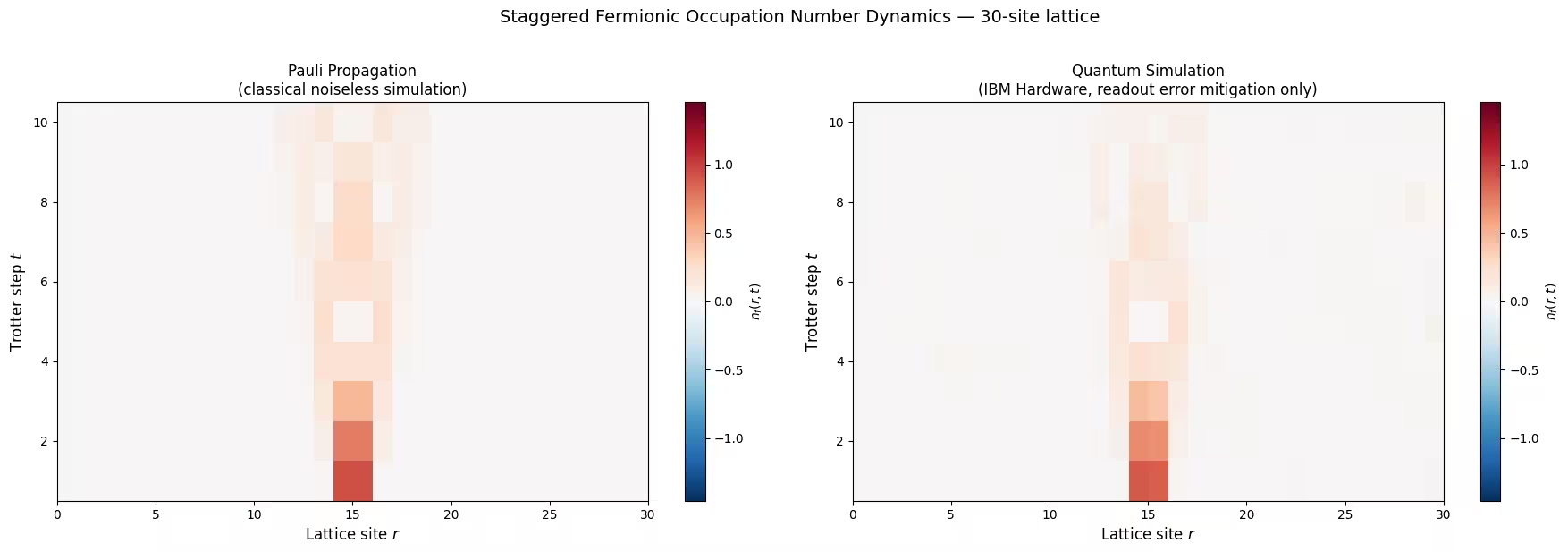
בנצ'מרקינג קלאסי באמצעות התפשטות פאולי
שיטת התפשטות פאולי (Pauli Propagation Method - PPM) מספקת סימולציה קלאסית נטולת רעש של ה-Circuit הקוונטי על ידי התפשטות אחורית של תצפיות נמדדות דרך ה-Circuit בתמונת הייזנברג. תחת שכבות קליפורד (Gate-ים מסוג CNOT, H, S, X), אופרטורי פאולי ממופים לאופרטורי פאולי אחרים ללא הגדלת מספר האיברים. שכבות לא-קליפורד (ה-Gate-ים מסוג במעגל) יכולות לגרום להסתעפות — במקרה הגרוע ביותר, הכפלת מספר האיברים — אך לענפים רבים יש מקדמים קטנים וניתן לקטום אותם.
תהליך העבודה עם pauli-prop הוא:
-
פיצול ה-Circuit לחלקי קליפורד ולא-קליפורד באמצעות
evolve_through_cliffords. -
התפשטות של כל תצפית דרך החלק הלא-קליפורדי באמצעות
propagate_through_circuit, תוך שמירה על עדmax_termsאיברי פאולי והשמטת איברים עם מקדמים מתחת לסף הקיטוםatol. -
התפתחות של התוצאה דרך החלק הקליפורדי באמצעות תמיכת הקליפורד המובנית של Qiskit.
-
חילוץ ערך התוחלת על ידי סכימת מקדמים של איברי פאולי אלכסוניים (המכילים רק ו-).
סף קיטום
הפרמטר atol ב-propagate_through_circuit שולט במידת האגרסיביות שבה ענפי פאולי קטנים נקטמים. סף הדוק מאוד (למשל, 1e-12) שומר כמעט על כל הענפים ונותן תוצאות מדויקות, אך זמן הסימולציה גדל בתלילות עם עומק ה-Circuit; הסימולציה בת 120 ה-Qubit-ים במאמר לקחה כ-8.5 שעות עם ההגדרות המוגדרות כברירת מחדל. העלאת הסף (למשל, ל-1e-6 או 1e-3) משמיטה איברים שהמקדמים שלהם נופלים מתחת לערך זה, ומפחיתה באופן דרמטי את מספר האיברים הנעקבים ומאיצה את החישוב. הפשרה היא שגיאת קירוב קטנה וניתנת לשליטה, שניתן לאמת אותה על ידי השוואת תוצאות בספים שונים.
import time
from pauli_prop import evolve_through_cliffords, propagate_through_circuit

# ── PPM Configuration ──
# Truncation threshold: controls the speed/accuracy trade-off.
PPM_THRESHOLD = 1e-3

# Maximum Pauli terms to track per observable (hard cap on memory/time)
PPM_MAX_TERMS = 66_000

print(f"PPM settings: atol={PPM_THRESHOLD}, max_terms={PPM_MAX_TERMS}")

# We propagate each single-qubit Z observable through each circuit.
# For PPM, we work with the un-transpiled circuits (ideal noiseless simulation).

observables_pp = [
    SparsePauliOp("I" * i + "Z" + "I" * (num_qubits_hw - i - 1))
    for i in range(num_qubits_hw)
]

def ppm_expectation_values(
    circuit, observables, max_terms=PPM_MAX_TERMS, atol=PPM_THRESHOLD
):
    """Compute expectation values of single-qubit Z observables
    via Pauli propagation.

    Args:
        circuit: The quantum circuit to simulate.
        observables: List of single-qubit Z observables.
        max_terms: Maximum number of Pauli terms to retain (hard cap).
        atol: Absolute tolerance — Pauli terms with coefficients below this
              value are discarded during propagation. Larger values give
              faster simulation at the cost of approximation accuracy.
    """
    circuit = circuit.decompose(["swap"])  # decompose SWAPs into 3 CX gates
    cliff, non_cliff = evolve_through_cliffords(circuit)

    evs = []
    for obs in observables:
        evolved_obs = propagate_through_circuit(
            obs, non_cliff, max_terms=max_terms, atol=atol, frame="h"
        )[0]
        evolved_obs.paulis = evolved_obs.paulis.evolve(cliff, frame="h")
        diagonal_mask = ~evolved_obs.paulis.x.any(axis=1)
        ev = float(evolved_obs.coeffs[diagonal_mask].sum().real)
        evs.append(ev)
    return np.array(evs)

# Run PPM for each Trotter step and record wall-clock time
pp_expvals_mid = []
pp_expvals = []
pp_times = []

for idx, d in enumerate(trotter_steps_hw):
    t_start = time.perf_counter()

    # Meson circuit
    evs_mid = ppm_expectation_values(circuits_mid_hw[idx], observables_pp)

    # Vacuum circuit
    evs_vac = ppm_expectation_values(circuits_hw[idx], observables_pp)

    elapsed = time.perf_counter() - t_start
    pp_times.append(elapsed)

    pp_expvals_mid.append(evs_mid[::-1])
    pp_expvals.append(evs_vac[::-1])

    print(f"Trotter step {d:2d}: {elapsed:.1f} s")

print(f"\nTotal PPM simulation time: {sum(pp_times):.1f} s")
print(f"Truncation threshold used: {PPM_THRESHOLD}")
PPM settings: atol=0.001, max_terms=66000
Trotter step  1: 5.0 s
Trotter step  2: 7.5 s
Trotter step  3: 11.2 s
Trotter step  4: 14.7 s
Trotter step  5: 18.3 s
Trotter step  6: 22.1 s
Trotter step  7: 25.6 s
Trotter step  8: 29.4 s
Trotter step  9: 33.2 s
Trotter step 10: 36.6 s

Total PPM simulation time: 203.6 s
Truncation threshold used: 0.001
# --- PPM simulation time vs. Trotter steps ---
fig, ax = plt.subplots(figsize=(8, 5))
ax.plot(
    list(trotter_steps_hw),
    pp_times,
    "o-",
    color="tab:blue",
    linewidth=2,
    markersize=6,
)
ax.set_xlabel("Trotter step", fontsize=13)
ax.set_ylabel("Wall-clock time (s)", fontsize=13)
ax.set_title(
    "Pauli Propagation simulation time vs. Trotter steps\n(30-site lattice, 60 qubits)",
    fontsize=13,
)
ax.grid(True, alpha=0.3)
plt.tight_layout()
plt.show()

# --- PPM heatmap and comparison with hardware ---
N_mid_pp = get_number(pp_expvals_mid, num_lattice_point_hw)
N_pp = get_number(pp_expvals, num_lattice_point_hw)
N_diff_pp = calculate_difference(N_mid_pp, N_pp, num_lattice_point_hw)

N_diff_pp_arr = np.array(N_diff_pp)

fig, axes = plt.subplots(1, 2, figsize=(18, 6))
vmax = np.abs(N_hw).max()
vmin = -vmax
norm = TwoSlopeNorm(vmin=vmin, vcenter=0, vmax=vmax)

# PPM result
im0 = axes[0].imshow(
    N_diff_pp_arr,
    aspect="auto",
    origin="lower",
    cmap="RdBu_r",
    norm=norm,
    extent=[0, num_lattice_point_hw, 0.5, len(trotter_steps_hw) + 0.5],
)
axes[0].set_xlabel("Lattice site $r$", fontsize=12)
axes[0].set_ylabel("Trotter step $t$", fontsize=12)
axes[0].set_title(
    "Pauli Propagation\n(classical noiseless simulation)", fontsize=12
)
plt.colorbar(im0, ax=axes[0], label="$n_f(r,t)$")

# Hardware result
im1 = axes[1].imshow(
    N_diff_hw_arr,
    aspect="auto",
    origin="lower",
    cmap="RdBu_r",
    norm=norm,
    extent=[0, num_lattice_point_hw, 0.5, len(trotter_steps_hw) + 0.5],
)
axes[1].set_xlabel("Lattice site $r$", fontsize=12)
axes[1].set_ylabel("Trotter step $t$", fontsize=12)
axes[1].set_title(
    "Quantum Simulation\n(IBM Hardware, readout error mitigation only)",
    fontsize=12,
)
plt.colorbar(im1, ax=axes[1], label="$n_f(r,t)$")

plt.suptitle(
    "Staggered Fermionic Occupation Number Dynamics — 30-site lattice",
    fontsize=14,
    y=1.02,
)
plt.tight_layout()
plt.show()
צעדים הבאים
אם עבודה זו עניינה אתכם, שקלו לחקור את החומר הבא:
-
תיעוד הפרימיטיב Estimator של Qiskit — לפרטים על הגדרת אפשרויות הקלת שגיאות
-
טכניקות הקלה ודיכוי שגיאות — ללמוד על TREX, ZNE ושיטות הקלה אחרות
-
Qiskit Pauli Propagation (pauli-prop) — סימולציה קלאסית מואצת ב-Rust באמצעות התפשטות אחורית של פאולי
מקורות
[1] המאמר המקורי: Ilčić, Majumdar, Mathew et al. "Observation of Robust and Coherent Non-Abelian Hadron Dynamics on Noisy Quantum Processors" arXiv:2602.18080 (2026)