סימולציית פיזור נייטרונים בחומרים קוונטיים עם מעגלים קוונטיים

אומדן שימוש: 13 דקות על מעבד Heron r2 (הערה: זהו אומדן בלבד. זמן הריצה שלך עשוי להשתנות.)

באיזה מדריך כדאי להשתמש?

השתמשו במדריך זה כדי ללמוד את היישום שלב אחר שלב, כאשר חישוב קלאסי רץ באופן מקומי על המחשב הנייד שלכם וביצוע חומרה על QPU של IBM Quantum®. הדוגמה בקנה מידה גדול דורשת זיכרון משמעותי, והידור קוונטי מקורב (AQC) יכול לקחת מספר שעות על משאבי מחשב נייד טיפוסיים. כדי להעביר את הדחיסה למשאבי המחשוב והזיכרון של Qiskit Serverless, השתמשו במדריך ה-Serverless הנלווה.

תוצאות למידה

כיצד ספקטרומי פיזור נייטרונים לא אלסטי (INS) מתקשרים לגורמי מבנה דינמיים (DSF) של מודלי ספין קוונטיים.
כיצד להכין מצב יסוד, להחיל הפרעה מקומית, ולבצע אבולוציית זמן טרוטר על מעגל קוונטי.
כיצד להשתמש בהידור קוונטי מקורב (AQC) עם qiskit-addon-aqc-tensor כדי לדחוס מעגלי טרוטר עמוקים לביצוע על חומרה.
כיצד לחלץ את פונקציית גרין המושהית (RGF) מערכי תוחלת קיוביטים ולבצע עליה התמרת פורייה לתוך DSF.

דרישות מוקדמות

רקע

במדריך זה, אנו משחזרים את התוצאות של Lee et al., arXiv:2603.15608.

פיזור נייטרונים מסייע לחוקרים לאפיין חומרים הרלוונטיים לקיימות, כולל אלקטרודות לסוללות. מדריך זה בוחן כיצד Circuit קוונטיים יכולים לדמות עוררויות מגנטיות ולקשר בין מודלים תיאורטיים למדידות פיזור. דוגמת המגנט הקוונטי שבמדריך מפתחת שיטות לחקר התנהגות חומרים, ותורמת לערכת הכלים הרחבה יותר של מחקר לגילוי חומרים.

פיזור נייטרונים לא אלסטי וגורם המבנה הדינמי

פיזור נייטרונים לא אלסטי (INS) הוא אחד מהחקרים הניסיוניים העוצמתיים ביותר של עירורים מגנטיים בחומרים קוונטיים. כאשר קרן של נייטרונים תרמיים או קרים פוגעת בגביש, נייטרונים בודדים מחליפים גם תנע $\mathbf{q}$ וגם אנרגיה $\omega$ עם תת-המערכת המגנטית. עוצמת הפיזור הנמדדת פרופורציונלית לגורם המבנה הדינמי (DSF),

$S^{\alpha\beta}(q,\omega) = \sum_{j} e^{-iq\,j}\int_{-\infty}^{\infty} dt\; e^{i\omega t}\, \langle S_0^{\alpha}(0)\, S_j^{\beta}(t)\rangle,$

אשר מקודד את מלוא המתאמים במרחב-זמן של דרגות החופש של הספין.

KCuF $_3$ : מגנט Luttinger-liquid קנוני

פלואוריד נחושת-אשלגן (KCuF $_3$ ) הוא אנטיפרומגנט כמעט חד-ממדי שבו שרשראות של יוני Cu $^{2+}$ בעלי ספין- $\frac{1}{2}$ מתקשרים באמצעות חילופי הייזנברג של שכנים קרובים $J$ , בעוד הצימוד הבין-שרשרתי הוא רק כ- $\sim 2.7\%$ מ- $J$ . ב- $T = 6\;\mathrm{K}$ שבו זמינים נתוני INS, הספקטרום נשלט על ידי עירורי ספינון מפוצלים האופייניים לנוזל Tomonaga-Luttinger. מכיוון שהדינמיקה התוך-שרשרתית מתוארת היטב על ידי האמילטוניאן XXZ החד-ממדי בעל ספין- $\frac{1}{2}$ בנקודה האיזוטרופית ( $\epsilon = 1$ ),

$H = J\sum_{i}\left[S_i^Z S_{i+1}^Z + \epsilon\left(S_i^X S_{i+1}^X + S_i^Y S_{i+1}^Y\right)\right],$

KCuF $_3$ משמש כמדד ביצועים אידיאלי לסימולציה קוונטית: האמילטוניאן פשוט מספיק כדי ליישום על מעבד קוונטי, אך מצב היסוד שזור בחוזקה וספקטרום העירורים כולל רצף דו-ספינוני רחב.

הערה: מדריך זה קובע $J = 1$ כיחידת האנרגיה ומאמץ את הנרמול $H = J\sum_i[\ldots]$ , אשר מתאים להאמילטוניאן המקומי $H_\mathrm{loc} = J(S^X S^X + S^Y S^Y + S^Z S^Z)$ המשמש בהמימוש המעגלי של המאמר (איור S3 של החומר המשלים). האמילטוניאן המלא של המאמר (משוואה 3) נושא גורם כללי נוסף של 2, כך שה- $J$ של המאמר הוא כפול מה- $J$ המשמש כאן.

מה אנו מסמלצים ומודדים

הגודל הפיזיקלי שאנו מחשבים הוא פונקציית גרין המושהית (RGF), המוגדרת כפונקציית המתאם ספין-ספין התלויה בזמן

$G^R_{\alpha,\beta}(j, j_c, t) = -\frac{i}{2}\,\langle\psi_{\mathrm{GS}}|\,S_j^\alpha(t)\,S_{j_c}^\beta(0) - S_{j_c}^\beta(0)\,S_j^\alpha(t)\,|\psi_{\mathrm{GS}}\rangle,$

כאשר $j_c$ הוא אתר ייחוס (מרכז השרשרת) ו- $S_j^\alpha(t) = e^{iHt}S_j^\alpha e^{-iHt}$ הוא אופרטור הספין בייצוג הייזנברג. במדריך זה אנו מתמקדים ברכיב ה- $zz$ ( $\alpha = \beta = z$ ). על מחשב קוונטי ניגשים ל-RGF על ידי הכנת מצב היסוד, החלת הפרעה מקומית ב- $j_c$ , אבולוציית זמן של המצב המופרע, ומדידת ערך התוחלת חד-קיוביט $\langle\sigma_j^z\rangle$ בכל אתר $j$ לכל צעד זמן. התובנה המרכזית היא שכל $\langle\sigma_j^z\rangle$ נותן את ההפרש ממגנטיזציית מצב היסוד; מכיוון שלאנטיפרומגנט הייזנברג האיזוטרופי יש מגנטיזציה נטו אפסית לכל אתר ( $\langle\sigma_j^z\rangle_\mathrm{GS} = 0$ ), הערך שנמדד ישירות נותן את $G^R(j, j_c, t)$ ללא כל חיסור מפורש.

על ידי איסוף $G^R(j, j_c, t)$ על פני כל האתרים וצעדי הזמן, אנו מרכיבים מערך נתונים דו-ממדי שעליו מבוצעת לאחר מכן התמרת פורייה הן במרחב והן בזמן כדי לייצר את גורם המבנה הדינמי $S(q,\omega)$ . ה-DSF הוא הגודל הנמדד ישירות בניסוי INS: הוא מספר לנו אילו עירורים מגנטיים קיימים בכל תנע $q$ ואנרגיה $\omega$ . עבור השרשרת הייזנברג האיזוטרופית, ספקטרום העירורים המדויק הוא רצף דו-ספינוני, רצועה רחבה של עוצמת פיזור שצורתה משמשת כמדד ביצועים קפדני מקצה לקצה לסימולציה הקוונטית: הוא מאמת את הכנת מצב היסוד, ההפרעה, אבולוציית הזמן טרוטר, ופרוטוקול המדידה כולם בבת אחת.

זרימת עבודה של סימולציה קוונטית

זרימת העבודה משקפת את הפיזיקה של אירוע INS. אנו (1) מכינים את מצב היסוד רב-הגוף $|\psi_{\mathrm{GS}}\rangle$ על $n$ קיוביטים, (2) מחילים הפרעת היפוך ספין מקומית $U_{j_c} = \frac{1}{\sqrt{2}}(I - i\sigma^z_{j_c})$ במרכז השרשרת כדי לחקות את העברת הספין של הנייטרון, (3) מבצעים אבולוציה תחת $H$ עבור צעדי זמן בדידים באמצעות טרוטריזציה מסדר שני, ו-(4) מודדים $\langle\sigma_i^z\rangle$ בכל קיוביט בכל צעד כדי לקבל את ה-RGF. התמרת פורייה בדידה דו-ממדית נותנת לאחר מכן את ה-DSF $S(q,\omega)$ .

הגודל הנצפה שאנו מודדים בכל צעד זמן הוא $\sigma_i^z$ על כל קיוביט $i$ . ב-Qiskit זה מיוצג כרשימה של אופרטורי SparsePauliOp: $Z$ חד-קיוביט אחד משוקע במחרוזת הזהות בת $n$ הקיוביטים עבור כל אתר. גדלים נצפים אלה נבנים פעם אחת עבור כל מופע בעיה במהלך שלב מיפוי הבעיה (שלב 1) ומשמשים שוב לכל מעגל בקנה מידה זה.

הידור קוונטי מקורב (AQC)

מעגלי טרוטר עמוקים ניתנים לדחיסה עם הידור קוונטי מקורב (AQC), אשר מחליף את שכבות הטרוטר הראשונות עם אנסאץ פרמטרי קצר יותר שהפרמטרים שלו מותאמים קלאסית כדי למקסם את הנאמנות ברמת ה-MPS עם המעגל העמוק המקורי. צעדי הטרוטר הנותרים מתווספים באופן מדויק, ומייצרים מעגל AQC + טרוטר "מעורב" עם פחות שערים דו-קיוביטיים באופן משמעותי.

סימולציית MPS

עבור מערכת חד-ממדית, שיטות מצב-מכפלת-מטריצות (MPS) יכולות לדמות ביעילות הן הכנת מצב יסוד (עם חבורת הרנורמליזציה של מטריצת הצפיפות, DMRG) והן אבולוציית זמן ברמת המעגל. על ידי שליטה בממד הקשר $\chi$ , אנו מאזנים בין דיוק לעלות חישובית. במדריך זה אנו משתמשים בסימולציית MPS בתוך qiskit-addon-aqc-tensor כדי לחשב אנסאצים AQC בעלי נאמנות גבוהה שדוחסים את מעגלי הטרוטר העמוקים לביצוע על חומרה.

דרישות

לפני שתתחיל במדריך זה, ודא שהתקנת את הדברים הבאים:

Qiskit SDK עם תמיכת ויזואליזציה
Qiskit Runtime (pip install qiskit-ibm-runtime)
qiskit-addon-aqc-tensor עם תוספי quimb ו-JAX (pip install 'qiskit-addon-aqc-tensor[quimb-jax]')

הגדרה

# Added by doQumentation — installs the packages this notebook needs if they are missing
import importlib.util

_needed = {"matplotlib": "matplotlib", "numpy": "numpy", "qiskit": "qiskit", "qiskit_addon_aqc_tensor": "qiskit-addon-aqc-tensor", "qiskit_ibm_runtime": "qiskit-ibm-runtime", "qiskit_quimb": "qiskit-quimb", "quimb": "quimb", "scipy": "scipy"}
_missing = [pip for module, pip in _needed.items()
            if importlib.util.find_spec(module) is None]
# One at a time, so a package that fails to install does not block the others
for _pip in _missing:
    %pip install -q {_pip}
if not _missing:
    print("\u2713 All required packages are installed")

import timeit
import warnings
from collections.abc import Iterator, Sequence
from functools import partial

import matplotlib.pyplot as plt
import numpy as np
import quimb.tensor as qtn
import scipy.optimize
from numpy.typing import NDArray
from qiskit import QuantumCircuit
from qiskit.circuit import CircuitInstruction, ParameterVector, Qubit
from qiskit.circuit.library import PauliEvolutionGate
from qiskit.primitives import StatevectorEstimator
from qiskit.quantum_info import SparsePauliOp
from qiskit.transpiler.preset_passmanagers import generate_preset_pass_manager
from qiskit_addon_aqc_tensor import generate_ansatz_from_circuit
from qiskit_addon_aqc_tensor.objective import MaximizeStateFidelity
from qiskit_addon_aqc_tensor.simulation import tensornetwork_from_circuit
from qiskit_addon_aqc_tensor.simulation.quimb import QuimbSimulator
from qiskit_ibm_runtime import EstimatorV2 as Estimator
from qiskit_ibm_runtime import QiskitRuntimeService
from qiskit_quimb import quimb_circuit
from scipy.sparse import SparseEfficiencyWarning

# scipy.sparse.linalg.expm (reached via PauliEvolutionGate.to_matrix) prefers
# CSC and warns when handed the CSR matrix from SparsePauliOp.to_matrix; the
# result is unaffected, so silence the cosmetic warning.
warnings.filterwarnings("ignore", category=SparseEfficiencyWarning)

def xxz_hamiltonian_mpo(
    n_qubits: int, interaction: float = 1.0, anisotropy: float = 1.0
) -> qtn.MatrixProductOperator:
    """1D XXZ Hamiltonian as a quimb MPO.

    Builds the Hamiltonian using ``qtn.SpinHam1D``.

    Args:
        n_qubits: Number of sites.
        interaction: Overall interaction strength (J in the paper).
        anisotropy: XY/Z anisotropy (ε in the paper). ``ε = 1`` is the
            isotropic Heisenberg point; ``ε = 0`` is the Ising limit.

    Returns:
        The Hamiltonian as a matrix product operator.
    """
    builder = qtn.SpinHam1D(S=1 / 2)
    builder += interaction * anisotropy * 0.5, "+", "-"
    builder += interaction * anisotropy * 0.5, "-", "+"
    builder += interaction, "Z", "Z"
    return builder.build_mpo(L=n_qubits)

def build_ground_state_ansatz(n_qubits: int, n_layers: int) -> QuantumCircuit:
    """Hamiltonian variational ansatz (HVA) circuit for ground-state preparation.

    Starts from a product of singlet pairs and applies alternating
    odd/even layers of parameterized XXZ pair-evolution gates.

    The returned circuit is parameterized: it carries a ``ParameterVector``
    named ``"theta"`` of length ``2 * n_layers`` whose values must be
    assigned (e.g. via ``circuit.assign_parameters``) before simulation.
    Element ``2 * r`` is the odd-layer angle and element ``2 * r + 1`` is the
    even-layer angle of layer ``r``.

    Args:
        n_qubits: Number of qubits (must be even).
        n_layers: Number of HVA layers.

    Returns:
        The parameterized HVA preparation circuit.
    """
    theta = ParameterVector("theta", 2 * n_layers)
    circuit = QuantumCircuit(n_qubits)
    # Initial singlet product state
    for i in range(n_qubits // 2):
        circuit.x(2 * i)
        circuit.x(2 * i + 1)
        circuit.h(2 * i + 1)
        circuit.cx(2 * i + 1, 2 * i)
    # Variational layers: each pair gate is exp(-i theta (XX+YY+ZZ)/2)
    pair_ham = SparsePauliOp(
        ["XX", "YY", "ZZ"], coeffs=[0.5, 0.5, 0.5]
    )  # H_pair (HVA form)
    for r in range(n_layers):
        for i in range(1, (n_qubits + 1) // 2):  # odd layer
            circuit.append(
                PauliEvolutionGate(pair_ham, time=theta[2 * r]),
                [2 * i - 1, 2 * i],
            )
        for i in range(n_qubits // 2):  # even layer
            circuit.append(
                PauliEvolutionGate(pair_ham, time=theta[2 * r + 1]),
                [2 * i, 2 * i + 1],
            )
    return circuit

def optimize_ground_state_ansatz(
    ansatz: QuantumCircuit,
    x0: NDArray[np.floating],
    target_mps: qtn.MatrixProductState,
    *,
    max_bond: int | None = None,
    cutoff: float = 1e-10,
    method: str = "COBYQA",
    options: dict | None = None,
) -> scipy.optimize.OptimizeResult:
    """Optimize HVA parameters by maximizing fidelity with a target MPS.

    The HVA circuit is simulated as a matrix product state with the given
    bond-dimension truncation, and the parameters are optimized to maximize
    the state fidelity ``|<psi_HVA | target_mps>|**2`` with the DMRG ground
    state. Both states are normalized, so the minimized objective is the
    infidelity ``1 - |<psi_HVA | target_mps>|**2``.

    Args:
        ansatz: Parameterized HVA circuit from ``build_ground_state_ansatz``.
            The length of ``x0`` must equal ``ansatz.num_parameters``.
        x0: Initial parameters.
        target_mps: Target MPS (DMRG ground state) to maximize fidelity with.
        max_bond: Maximum MPS bond dimension during gate application.
        cutoff: Singular-value cutoff during gate application.
        method: ``scipy.optimize.minimize`` method.
        options: Options dict forwarded to ``scipy.optimize.minimize``.

    Returns:
        The Scipy OptimizeResult.
    """

    def infidelity(params: NDArray[np.floating]) -> float:
        circuit = ansatz.assign_parameters(params)
        circuit_mps = quimb_circuit(
            circuit.decompose(["PauliEvolution"]),
            quimb_circuit_class=qtn.CircuitMPS,
            max_bond=max_bond,
            cutoff=cutoff,
        )
        return 1 - abs(circuit_mps.psi.H @ target_mps) ** 2

    return scipy.optimize.minimize(
        infidelity, np.asarray(x0), method=method, options=options
    )

def trotter_evolution(
    qubits: Sequence[Qubit],
    interaction: float,
    anisotropy: float,
    time_step: float,
    n_steps: int,
) -> Iterator[CircuitInstruction]:
    """Second-order Trotter steps of the XXZ pair Hamiltonian.

    While the paper used a hand-optimized circuit for the Trotter steps, we use
    PauliEvolutionGate here for simplicity and generality. The final two-qubit gate
    count and gate depth are equivalent when transpiled with ``optimization_level=3``.

    Args:
        qubits: Qubits to act on (length ``n_qubits``).
        interaction: Overall interaction strength (J in the paper).
        anisotropy: XY/Z anisotropy (ε in the paper). ``ε = 1`` is the
            isotropic Heisenberg point; ``ε = 0`` is the Ising limit.
        time_step: Per-step Trotter time.
        n_steps: Number of Trotter steps.

    Yields:
        ``CircuitInstruction``s implementing the Trotter steps.
    """
    if n_steps == 0:
        return
    n_qubits = len(qubits)
    pair_ham = SparsePauliOp(
        ["XX", "YY", "ZZ"],
        coeffs=[
            0.25 * interaction * anisotropy,
            0.25 * interaction * anisotropy,
            0.25 * interaction,
        ],
    )
    half_evo = PauliEvolutionGate(pair_ham, time=time_step / 2)
    full_evo = PauliEvolutionGate(pair_ham, time=time_step)
    for i in range(n_qubits // 2):  # half even layer
        yield CircuitInstruction(half_evo, (qubits[2 * i], qubits[2 * i + 1]))
    for i in range(n_qubits // 2 - 1):  # full odd layer
        yield CircuitInstruction(
            full_evo, (qubits[2 * i + 1], qubits[2 * i + 2])
        )
    for _ in range(n_steps - 1):  # interior steps
        for i in range(n_qubits // 2):
            yield CircuitInstruction(
                full_evo, (qubits[2 * i], qubits[2 * i + 1])
            )
        for i in range(n_qubits // 2 - 1):
            yield CircuitInstruction(
                full_evo, (qubits[2 * i + 1], qubits[2 * i + 2])
            )
    for i in range(n_qubits // 2):  # half even layer
        yield CircuitInstruction(half_evo, (qubits[2 * i], qubits[2 * i + 1]))

def get_dsf(
    n_qubits: int,
    rgf_mat: NDArray[np.floating],
    time_step: float,
    n_steps: int,
    n_points_momentum: int,
    n_points_frequency: int,
) -> NDArray[np.floating]:
    """Compute the dynamical structure factor from the retarded Green's function.

    Uses the center-site approximation and a discrete Fourier transform.
    The result is symmetrized about the momentum axis and clipped to
    non-negative values, ready for plotting.

    Args:
        n_qubits: Number of qubits (sites).
        rgf_mat: RGF matrix of shape ``(n_steps, n_qubits)``.
        time_step: Trotter time-step size.
        n_steps: Number of time steps.
        n_points_momentum: Number of momentum points.
        n_points_frequency: Number of frequency points.

    Returns:
        DSF array of shape ``(n_points_frequency, n_points_momentum)``,
        symmetrized about the momentum axis and clipped to non-negative values.
    """
    max_frequency = np.pi / time_step
    momentum_range = np.linspace(0, 2 * np.pi, n_points_momentum)
    frequency_range = np.linspace(0, max_frequency, n_points_frequency)
    result = np.zeros((frequency_range.shape[0], momentum_range.shape[0]))
    center = n_qubits // 2 - 1
    for iw, w in enumerate(frequency_range):
        exponent = np.exp(1j * w * time_step * np.arange(1, n_steps + 1))
        # S = sigma/2, so two spin operators contribute a factor of (1/2)(1/2) = 1/4.
        rgf_omega = (
            np.dot(rgf_mat.T, exponent) * time_step / 4
        )  # S(omega): time Fourier slice of the Green's function
        for iq, q in enumerate(momentum_range):
            momentum_phases = np.exp(
                -1j * q * np.arange(-center, center + 2, 1)
            )
            result[iw, iq] = np.imag(np.dot(rgf_omega, momentum_phases))
    result = -(result + result[:, ::-1]) / 2
    result = np.clip(result, a_min=0, a_max=None)
    return result

def plot_dsf(
    dsf: NDArray[np.floating],
    time_step: float,
    n_points_momentum: int,
    n_points_frequency: int,
    title: str | None = None,
) -> None:
    """Heat-map of the dynamical structure factor.

    Args:
        dsf: DSF array of shape ``(n_points_frequency, n_points_momentum)``.
        time_step: Trotter time-step size.
        n_points_momentum: Number of momentum points.
        n_points_frequency: Number of frequency points.
        title: Optional plot title.
    """
    max_frequency = np.pi / time_step
    momentum_range = np.linspace(0, 2 * np.pi, n_points_momentum)
    frequency_range = np.linspace(0, max_frequency, n_points_frequency)
    x, y = np.meshgrid(momentum_range, frequency_range)
    fig, ax = plt.subplots(figsize=(8, 5))
    c = ax.pcolormesh(x, y, dsf / np.max(dsf), cmap="viridis", shading="auto")
    fig.colorbar(c, ax=ax, label="Normalized intensity")
    ax.set_ylim(0, 3.6)
    ax.set_xlim(0, 2 * np.pi)
    ax.set_xlabel(r"$q$", fontsize=16)
    ax.set_ylabel(r"$\tilde{\omega} = \omega / J$", fontsize=16)
    ax.set_xticks([0, np.pi / 2, np.pi, 3 * np.pi / 2, 2 * np.pi])
    ax.set_xticklabels(["0", r"$\pi/2$", r"$\pi$", r"$3\pi/2$", r"$2\pi$"])
    if title:
        ax.set_title(title, fontsize=14)
    plt.tight_layout()
    plt.show()

def plot_rgf(
    n_qubits: int,
    rgf_mat: NDArray[np.floating],
    time_step: float,
    n_steps: int,
    title: str | None = None,
) -> None:
    """Heat-map of the retarded Green's function in real space and time.

    Args:
        n_qubits: Number of qubits (sites).
        rgf_mat: RGF matrix of shape ``(n_steps, n_qubits)``.
        time_step: Trotter time-step size.
        n_steps: Number of time steps.
        title: Optional plot title.
    """
    fig, ax = plt.subplots(figsize=(8, 6))
    qubit_axis = np.arange(n_qubits)
    t_axis = np.arange(1, n_steps + 1) * time_step
    x, y = np.meshgrid(qubit_axis, t_axis)
    c = ax.pcolormesh(
        x,
        y,
        np.real(rgf_mat),
        cmap="RdBu",
        vmax=0.5,
        vmin=-0.5,
        shading="auto",
    )
    fig.colorbar(c, ax=ax, label=r"Re $G^R(j, j_c, t)$")
    ax.set_xlabel("Qubit", fontsize=16)
    ax.xaxis.set_major_locator(
        plt.matplotlib.ticker.MaxNLocator(integer=True)
    )
    ax.set_ylabel(r"Time", fontsize=16)
    if title:
        ax.set_title(title, fontsize=14)
    plt.tight_layout()
    plt.show()

def uniform_2q_depth(circuit: QuantumCircuit) -> int:
    """Two-qubit gate depth in a standardized basis."""
    pass_manager = generate_preset_pass_manager(
        optimization_level=0, basis_gates=["cz", "id", "rz", "sx", "x"]
    )
    return pass_manager.run(circuit).depth(
        lambda inst: inst.operation.num_qubits == 2
    )

דוגמת סימולטור בקנה מידה קטן

נדגים תחילה את זרימת העבודה המלאה על 10 קיוביטים, כאשר אנו מבצעים אופטימיזציה לאנסאץ מצב היסוד HVA באמצעות שימוש בסימולציית MPS ושימוש בסימולטור וקטור מצב של Qiskit לאבולוציית זמן. DMRG נותן אנרגיית מצב יסוד ייחוס ו-MPS ייחוס. דוגמה בקנה מידה קטן זו מאפשרת לנו לאמת כל צעד לפני שמגדילים את קנה המידה.

שלב 1: מיפוי קלטים קלאסיים לבעיה קוונטית

נתחיל בהגדרת המודל הפיזיקלי ובנייה של המעגלים הקוונטיים.

האמילטוניאן. KCuF $_3$ מדומה על ידי האמילטוניאן XXZ החד-ממדי בנקודה האיזוטרופית ( $J = 1$ , $\epsilon = 1$ , תוך קביעת $J = 1$ כיחידת האנרגיה).

מצב יסוד. אנו משתמשים במעגל אנסאץ וריאציוני האמילטוניאן (HVA), build_ground_state_ansatz, כמעגל הכנת מצב היסוד. הפרמטרים של ה-HVA מותאמים קלאסית על ידי מיקסום נאמנות המצב $|\langle\psi_{\mathrm{HVA}}(\theta)|\psi_{\mathrm{DMRG}}\rangle|^2$ עם ה-MPS של מצב היסוד DMRG, כאשר מצב ה-HVA מוערך על ידי סימולציה של המעגל כמצב-מכפלת-מטריצות עם CircuitMPS של quimb. אנו משתמשים ב-scipy.optimize.minimize לאופטימיזציה. האנרגיה $\langle H \rangle$ של האנסאץ המותאם מחושבת גם היא לצורך ייחוס.

שערי טרוטר. כל איבר אינטראקציית שכנים קרובים $e^{-i\Delta t\, H_{\mathrm{pair}}}$ עם $H_{\mathrm{pair}} = (J/4)(XX + YY + ZZ)$ נבנה עם PauliEvolutionGate(H_pair, time=time_step). Qiskit מסנתז זאת לפירוק אופטימלי של שלושה CNOT במהלך התרגום.

הפרעה. שער $R_z(\pi/2)$ על הקיוביט המרכזי מיישם את $U_{j_c} = \frac{1}{\sqrt{2}}(I - i\sigma^z_{j_c})$ , ומחקה את היפוך הספין המקומי שמייצר נייטרון מפוזר.

גדלים נצפים. אנו בונים גודל נצפה $\sigma^z$ עבור כל אתר קיוביט. אובייקטי SparsePauliOp אלה מועברים ל-primitive של Estimator בשלב 3 כדי לחלץ את $\langle\sigma_i^z\rangle$ בכל צעד זמן.

# -- Physical parameters --
n_qubits = 10
interaction = 1.0  # J
anisotropy = 1.0  # ε (isotropic point)
time_step = 0.6
n_steps = 10
mps_max_bond = 32
mps_cutoff = 1e-8
center = n_qubits // 2 - 1

# -- Hamiltonian MPO --
ham_mpo = xxz_hamiltonian_mpo(n_qubits, interaction, anisotropy)

# -- Reference ground-state energy via DMRG --
dmrg = qtn.DMRG2(ham_mpo)
dmrg.solve(tol=1e-8)
print(f"Ground-state energy (DMRG): {dmrg.energy:.6f}")

# -- Build ground state ansatz circuit --
gs_n_layers = 3
gs_ansatz = build_ground_state_ansatz(n_qubits, gs_n_layers)

# -- Optimize ground state ansatz parameters to maximize fidelity with the DMRG MPS --
# Initialize odd-layer angles near 0 (where the inter-pair gate is the
# identity) and even-layer angles near pi/2 (where the intra-pair gate
# is a SWAP, since 0.5*(XX + YY + ZZ) = SWAP - I/2).
rng = np.random.default_rng(12345)
x0 = np.tile([0, np.pi / 2], gs_n_layers) + rng.normal(
    scale=0.1, size=2 * gs_n_layers
)
print("Optimizing ground state ansatz...")
t0 = timeit.default_timer()
result = optimize_ground_state_ansatz(
    gs_ansatz,
    x0,
    dmrg.state,
    max_bond=mps_max_bond,
    cutoff=mps_cutoff,
    options=dict(maxiter=100),
)
t1 = timeit.default_timer()
print(f"Finished optimizing ground state ansatz in {t1 - t0} seconds.")
print(f"Ground state ansatz fidelity: {1 - result.fun:.6f}")

gs_circuit = gs_ansatz.assign_parameters(result.x)
gs_circuit_mps = quimb_circuit(
    gs_circuit.decompose(["PauliEvolution"]),
    quimb_circuit_class=qtn.CircuitMPS,
    max_bond=mps_max_bond,
    cutoff=mps_cutoff,
)
gs_ansatz_energy = qtn.expec_TN_1D(
    gs_circuit_mps.psi.H, ham_mpo, gs_circuit_mps.psi
)
print(f"Ground state ansatz energy: {gs_ansatz_energy:.6f}")

# -- Build circuits for each time step --
perturbed = gs_circuit.copy()
perturbed.rz(np.pi / 2, center)

circuits = []
for t in range(1, n_steps + 1):
    circuit = perturbed.copy()
    for instr in trotter_evolution(
        circuit.qubits, interaction, anisotropy, time_step, t
    ):
        circuit.append(instr)
    circuits.append(circuit)
print(
    f"Built {len(circuits)} circuits, deepest 2q depth (uniform basis) = "
    f"{uniform_2q_depth(circuits[-1])}"
)

# -- Observables: Z on each qubit site --
observables = [
    SparsePauliOp.from_sparse_list([("Z", [i], 1)], num_qubits=n_qubits)
    for i in range(n_qubits)
]
print(f"Defined {len(observables)} Z observables.")

Ground-state energy (DMRG): -4.258035
Optimizing ground state ansatz...
Finished optimizing ground state ansatz in 8.850687621976249 seconds.
Ground state ansatz fidelity: 0.984277
Ground state ansatz energy: -4.232565
Built 10 circuits, deepest 2q depth (uniform basis) = 163
Defined 10 Z observables.

שלב 2: אופטימיזציה של הבעיה לביצוע על חומרה קוונטית

עבור חומרה אמיתית, מעגלי הטרוטר שלמעלה יהיו עמוקים מדי. הידור קוונטי מקורב (AQC) מטפל בכך על ידי החלפת $k$ שכבות הטרוטר הראשונות (כולל מעגל מצב היסוד) עם אנסאץ פרמטרי קצר יותר שמותאם כדי למקסם את הנאמנות ברמת ה-MPS עם המעגל העמוק המקורי. צעדי הטרוטר הנותרים מתווספים באופן מדויק, ומייצרים מעגל "AQC + טרוטר" רדוד יותר.

כדי לאזן בין ביטוייות לעומק מעגל, שני אנסאצים משמשים: אנסאץ בעל שכבה אחת (שנוצר מצעד טרוטר בודד) דוחס את צעדי הזמן המוקדמים ביותר, ואנסאץ עמוק יותר בעל שתי שכבות (שנוצר משני צעדי טרוטר) דוחס את הצעדים הבאים שבהם נדרשת נאמנות גבוהה יותר.

לזרימת העבודה של AQC יש ארבעה תת-שלבים:

בנה מעגלי יעד — $k_1 + k_2$ המעגלים הראשונים משלב 1 משמשים ישירות כיעדי AQC.
חשב MPS יעד — דמה כל מעגל יעד כמצב-מכפלת-מטריצות באמצעות quimb.tensor.CircuitMPS.
צור והתאם אנסאצים — generate_ansatz_from_circuit יוצר אנסאץ פרמטרי בעל שכבה אחת ואנסאץ בעל שתי שכבות; הפרמטרים מותאמים באמצעות שימוש ב-L-BFGS-B עם גרדיאנטים מואצי JAX כדי למזער $1 - |\langle\psi_{\mathrm{ansatz}}|\psi_{\mathrm{target}}\rangle|^2$ . $k_1$ הצעדים הראשונים משתמשים באנסאץ בעל שכבה אחת ו- $k_2$ הצעדים הבאים משתמשים באנסאץ בעל שתי שכבות; בתוך כל שלב, כל צעד מתחיל (warm start) מהפרמטרים המותאמים של הצעד הקודם, ובמעבר בין שלבים הפרמטרים מאופסים לברירות המחדל של השלב.
הרכב מעגלים מעורבים — עבור צעדי זמן שמעבר לנקודת הביקורת של AQC, הוסף שכבות טרוטר מדויקות למעגל ה-AQC המותאם בעל שתי השכבות באמצעות trotter_evolution.

# Number of time steps to compress into an AQC ansatz with one layer
aqc_n_steps_1 = 3
# Number of time steps to compress into an AQC ansatz with two layers
aqc_n_steps_2 = 2
aqc_n_steps_total = aqc_n_steps_1 + aqc_n_steps_2

# ── Step 2a: Target circuits (first aqc_n_steps_total circuits from Step 1) ──
target_circuits = {
    k: circuits[k - 1] for k in range(1, aqc_n_steps_total + 1)
}
# ── Step 2b: Compute target MPS ──
# Decompose PauliEvolutionGate to RXX/RYY/RZZ before passing to the AQC MPS
# backend, which does not understand PauliEvolutionGate natively.
aqc_sim = QuimbSimulator(
    quimb_circuit_factory=partial(
        qtn.CircuitMPS,
        gate_opts=dict(max_bond=mps_max_bond, cutoff=mps_cutoff),
    ),
    autodiff_backend="jax",
)
print("\nStep 2b — target MPS:")
target_mps = {}
for k in range(1, aqc_n_steps_total + 1):
    target_mps[k] = tensornetwork_from_circuit(
        target_circuits[k].decompose(["PauliEvolution"]), aqc_sim
    )
    print(f"  k={k}: max bond = {target_mps[k].psi.max_bond()}")

# ── Step 2c: Generate ansätze (one-layer and two-layer) and optimize parameters ──
ansatz_1, initial_params_1 = generate_ansatz_from_circuit(
    target_circuits[1].decompose(["PauliEvolution"]),
    qubits_initially_zero=True,
)
initial_params_1 = np.array(initial_params_1)
ansatz_2, initial_params_2 = generate_ansatz_from_circuit(
    target_circuits[2].decompose(["PauliEvolution"]),
    qubits_initially_zero=True,
)
initial_params_2 = np.array(initial_params_2)
print(
    f"\nStep 2c — one-layer ansatz: {ansatz_1.num_parameters} parameters, "
    f"2q depth (uniform basis) = {uniform_2q_depth(ansatz_1)}"
)
print(
    f"Step 2c — two-layer ansatz: {ansatz_2.num_parameters} parameters, "
    f"2q depth (uniform basis) = {uniform_2q_depth(ansatz_2)}"
)

aqc_circuits = {}
aqc_params = {}
for k in range(1, aqc_n_steps_total + 1):
    if k <= aqc_n_steps_1:
        ansatz, base_params = ansatz_1, initial_params_1
    else:
        ansatz, base_params = ansatz_2, initial_params_2
    # Warm-start from the previous step only within the same stage
    same_stage = (k - 1 >= 1) and (
        (k - 1 <= aqc_n_steps_1) == (k <= aqc_n_steps_1)
    )
    x0 = aqc_params[k - 1] if same_stage else base_params
    obj = MaximizeStateFidelity(target_mps[k], ansatz, aqc_sim)
    t0 = timeit.default_timer()
    result = scipy.optimize.minimize(
        obj.loss_function,
        x0,
        method="L-BFGS-B",
        jac=True,
        options=dict(maxiter=100),
    )
    elapsed = timeit.default_timer() - t0
    aqc_params[k] = result.x
    aqc_circuits[k] = ansatz.assign_parameters(result.x)
    print(
        f"  k={k}: fidelity = {1 - result.fun:.4f}, "
        f"2q depth (uniform basis) = "
        f"{uniform_2q_depth(aqc_circuits[k])}, "
        f"{elapsed:.1f}s"
    )

# ── Step 2d: Assemble full circuit set (AQC + Trotter) ──
all_circuits = []
for k in range(1, aqc_n_steps_total + 1):
    all_circuits.append(aqc_circuits[k])
base = aqc_circuits[aqc_n_steps_total]
for k in range(1, n_steps - aqc_n_steps_total + 1):
    circuit = base.copy()
    for instr in trotter_evolution(
        circuit.qubits, interaction, anisotropy, time_step, k
    ):
        circuit.append(instr)
    all_circuits.append(circuit)

full_depths = [
    uniform_2q_depth(circuits[k - 1]) for k in range(1, n_steps + 1)
]
aqc_depths = [uniform_2q_depth(circuit) for circuit in all_circuits]
full_2q = [
    circuits[k - 1].decompose(["PauliEvolution"]).num_nonlocal_gates()
    for k in range(1, n_steps + 1)
]
aqc_2q = [
    circuit.decompose(["PauliEvolution"]).num_nonlocal_gates()
    for circuit in all_circuits
]
print(f"\nStep 2d — assembled {len(all_circuits)} circuits")
print(
    f"  At step {n_steps} (uniform basis): "
    f"Trotter 2q depth = {full_depths[-1]}, AQC+Trotter 2q depth = {aqc_depths[-1]}; "
    f"2q gates: Trotter = {full_2q[-1]}, AQC+Trotter = {aqc_2q[-1]}"
)

steps_axis = np.arange(1, n_steps + 1)
fig, ax = plt.subplots(figsize=(7, 4))
ax.plot(steps_axis, full_depths, "-o", color="black", label="Full Trotter")
ax.plot(
    steps_axis, aqc_depths, "-o", color="cadetblue", label="AQC + Trotter"
)
ax.set_xlabel("Trotter steps", fontsize=13)
ax.xaxis.set_major_locator(plt.matplotlib.ticker.MaxNLocator(integer=True))
ax.set_ylabel("2q gate depth (uniform basis)", fontsize=13)
ax.set_title(f"AQC circuit-depth reduction ({n_qubits} qubits)", fontsize=13)
ax.legend(fontsize=11)
plt.tight_layout()
plt.show()

Step 2b — target MPS:
  k=1: max bond = 22
  k=2: max bond = 22
  k=3: max bond = 26
  k=4: max bond = 27
  k=5: max bond = 30

Step 2c — one-layer ansatz: 389 parameters, 2q depth (uniform basis) = 27
Step 2c — two-layer ansatz: 470 parameters, 2q depth (uniform basis) = 33
  k=1: fidelity = 1.0000, 2q depth (uniform basis) = 27, 11.8s
  k=2: fidelity = 0.9980, 2q depth (uniform basis) = 27, 13.2s
  k=3: fidelity = 0.9890, 2q depth (uniform basis) = 27, 13.7s
  k=4: fidelity = 0.9983, 2q depth (uniform basis) = 33, 16.4s
  k=5: fidelity = 0.9957, 2q depth (uniform basis) = 33, 16.4s

Step 2d — assembled 10 circuits
  At step 10 (uniform basis): Trotter 2q depth = 163, AQC+Trotter 2q depth = 99; 2q gates: Trotter = 371, AQC+Trotter = 200

Output of the previous code cell

שלב 3: ביצוע באמצעות Qiskit primitives

אנו מדמים כל מעגל שהודר על ידי AQC באמצעות ה-primitive StatevectorEstimator.

estimator = StatevectorEstimator()
pubs = [(circuit, observables) for circuit in all_circuits]
job = estimator.run(pubs)
result = job.result()

שלב 4: עבד ולאחר מכן החזר תוצאה בפורמט קלאסי רצוי

כעת נחלץ את ערך התוחלת $\langle\sigma_i^z\rangle$ עבור כל קיוביט $i$ בכל צעד זמן $t$ . ערכים אלה יוצרים את מטריצת פונקציית גרין המושהית $G^R(j, j_c, t)$ . לאחר מכן, אנו מבצעים התמרת פורייה של ה-RGF לתוך גורם המבנה הדינמי $S(q, \omega)$ ומציגים גם את ה-RGF וגם את ה-DSF. get_dsf מחילה סימטריית מראה וגוזרת ערכים שליליים באופן פנימי.

rgf_mat = np.stack([pub_result.data.evs for pub_result in result])

# -- Compute DSF --
n_points_momentum, n_points_frequency = 100, 100
spectrum = get_dsf(
    n_qubits,
    rgf_mat,
    time_step,
    n_steps,
    n_points_momentum,
    n_points_frequency,
)

# -- Plot retarded Green's function --
plot_rgf(
    n_qubits,
    rgf_mat,
    time_step,
    n_steps,
    title=f"Retarded Green's function — {n_qubits} qubits (simulation)",
)

# -- Plot DSF --
plot_dsf(
    spectrum,
    time_step,
    n_points_momentum,
    n_points_frequency,
    title=f"Dynamical structure factor — {n_qubits} qubits (simulation)",
)

Output of the previous code cell

ביצוע חומרה בקנה מידה גדול

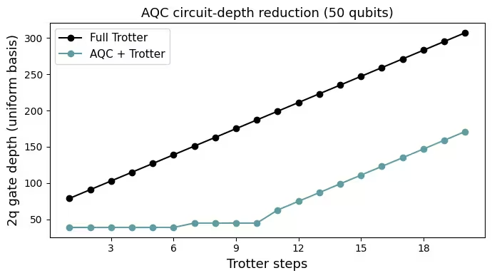
כעת נעלה בקנה מידה ל50 קיוביטים. בקנה מידה זה, האופטימיזציות מגיעות לנאמנויות נמוכות יותר מאשר בדוגמה בקנה מידה קטן: נאמנות אנסאץ מצב היסוד יורדת לבערך 0.65, ונאמנויות ה-AQC יורדות לבערך 0.7 בנקודות הביקורת המאוחרות יותר. זה צפוי, ותוכל לשפר נאמנויות אלה על ידי הגדלת מספר שכבות אנסאץ מצב היסוד (gs_n_layers) או מספר איטרציות האופטימיזציה (maxiter) במחיר קלאסי נוסף. שים לב גם שנאמנויות ה-AQC בעלות שתי השכבות יוצאות נמוכות יותר מאלה בעלות שכבה אחת. זו אינה נסיגה: צעדי זמן מאוחרים יותר מייצרים יותר שזירות ופשוט קשה יותר לדחוס אותם, ולכן האנסאץ בעל שתי השכבות המבטא יותר משמש עבורם.

אופטימיזציית ה-AQC יכולה גם לקחת מספר שעות של זמן חישוב קלאסי (בערך שש שעות בהרצה המוצגת כאן, רובן מושקעות בנקודות הביקורת בעלות שתי השכבות בשלב 2c). כדי לצמצם את זמן השעון הקיר, שקול להריץ מחברת זו על חומרה קלאסית עוצמתית יותר, כגון מערכת מחשוב בעלת ביצועים גבוהים (HPC). לחלופין, תוכל להקטין את קנה המידה לבעיה קטנה יותר (למשל, פחות קיוביטים או פחות צעדי זמן); התוצאות שלך יהיו אז שונות מאלה המוצגות כאן.

הקוד שלהלן עוקב אחר אותו מבנה בן ארבעה שלבים כמו בדוגמה בקנה המידה הקטן. פרמטרי מצב היסוד של ה-HVA מותאמים שוב באמצעות סימולציית MPS. על ה-QPU, אנו מפעילים ניתוק דינמי (DD), Pauli twirling, ו-twirled readout error extinction (TREX) לדיכוי והפחתת שגיאות. הטבלה הבאה מסכמת כיצד הניסוי בקנה מידה גדול שונה מזה בקנה מידה קטן:

	קנה מידה קטן	קנה מידה גדול
קיוביטים	10	50
צעדי זמן	10	20
נקודות ביקורת AQC (שכבה 1 + שכבה 2)	3 + 2 = 5	6 + 4 = 10
שכבות אנסאץ מצב יסוד	3	5
ממד קשר מקסימלי MPS	32	128
Estimator	`StatevectorEstimator`	QPU עם DD, טוויירלינג פאולי, ו-TREX

הודעות הידור איטי של XLA

במהלך אופטימיזציית ה-AQC (שלב 2c למטה) ייתכן שתראה הודעות stderr כגון:

[Compiling module jit_MakeArrayFn for CPU] Very slow compile? ...
The operation took 2m14s

אלה אבחונים שפירים מ-XLA, המהדר שעליו מבוסס ה-autodiff של JAX ב-qiskit-addon-aqc-tensor. ב-50 קיוביטים עם ממד קשר MPS 128, XLA מבלה כמה דקות בהידור פונקציית הגרדיאנט בפעם הראשונה שהיא נעקבת. ההידור מצליח, ותוצאות האופטימיזציה אינן מושפעות.

# ── Parameters ──────────────────────────────────────────────────────────────
n_qubits = 50  # 10 → 50
interaction = 1.0  # J
anisotropy = 1.0  # ε (isotropic point)
time_step = 0.6
n_steps = 20  # 10 → 20
aqc_n_steps_1 = 6  # 3 → 6
aqc_n_steps_2 = 4  # 2 → 4
aqc_n_steps_total = aqc_n_steps_1 + aqc_n_steps_2
gs_n_layers = 5  # 3 → 5
mps_max_bond = 128  # 32 -> 128
mps_cutoff = 1e-8
center = n_qubits // 2 - 1

# ── Step 1: Map ──────────────────────────────────────────────────────────────
ham_mpo = xxz_hamiltonian_mpo(n_qubits, interaction, anisotropy)

dmrg = qtn.DMRG2(ham_mpo)
dmrg.solve(tol=1e-8)
print(f"Ground-state energy (DMRG): {dmrg.energy:.6f}")

gs_ansatz = build_ground_state_ansatz(n_qubits, gs_n_layers)

rng = np.random.default_rng(12345)
x0 = np.tile([0.0, np.pi / 2], gs_n_layers) + rng.normal(
    scale=0.1, size=2 * gs_n_layers
)
print("Optimizing ground state ansatz...")
t0 = timeit.default_timer()
result = optimize_ground_state_ansatz(
    gs_ansatz,
    x0,
    dmrg.state,
    max_bond=mps_max_bond,
    cutoff=mps_cutoff,
    options=dict(maxiter=100),
)
t1 = timeit.default_timer()
print(f"Finished optimizing ground state ansatz in {t1 - t0} seconds.")
print(f"Ground state ansatz fidelity: {1 - result.fun:.6f}")

gs_circuit = gs_ansatz.assign_parameters(result.x)
gs_circuit_mps = quimb_circuit(
    gs_circuit.decompose(["PauliEvolution"]),
    quimb_circuit_class=qtn.CircuitMPS,
    max_bond=mps_max_bond,
    cutoff=mps_cutoff,
)
gs_ansatz_energy = qtn.expec_TN_1D(
    gs_circuit_mps.psi.H, ham_mpo, gs_circuit_mps.psi
)
print(f"Ground state ansatz energy: {gs_ansatz_energy:.6f}")

perturbed = gs_circuit.copy()
perturbed.rz(np.pi / 2, center)

circuits = []
for t in range(1, n_steps + 1):
    circuit = perturbed.copy()
    for instr in trotter_evolution(
        circuit.qubits, interaction, anisotropy, time_step, t
    ):
        circuit.append(instr)
    circuits.append(circuit)
print(
    f"Built {len(circuits)} circuits, deepest 2q depth (uniform basis) = "
    f"{uniform_2q_depth(circuits[-1])}"
)

observables = [
    SparsePauliOp.from_sparse_list([("Z", [i], 1)], num_qubits=n_qubits)
    for i in range(n_qubits)
]
print(f"Defined {len(observables)} Z observables.")

# ── Step 2: AQC ──────────────────────────────────────────────────────────────
target_circuits = {
    k: circuits[k - 1] for k in range(1, aqc_n_steps_total + 1)
}

aqc_sim = QuimbSimulator(
    quimb_circuit_factory=partial(
        qtn.CircuitMPS,
        gate_opts=dict(max_bond=mps_max_bond, cutoff=mps_cutoff),
    ),
    autodiff_backend="jax",
)
print("\nStep 2b — target MPS:")
target_mps = {}
for k in range(1, aqc_n_steps_total + 1):
    target_mps[k] = tensornetwork_from_circuit(
        target_circuits[k].decompose(["PauliEvolution"]), aqc_sim
    )
    print(f"  k={k}: max bond = {target_mps[k].psi.max_bond()}")

ansatz_1, initial_params_1 = generate_ansatz_from_circuit(
    target_circuits[1].decompose(["PauliEvolution"]),
    qubits_initially_zero=True,
)
initial_params_1 = np.array(initial_params_1)
ansatz_2, initial_params_2 = generate_ansatz_from_circuit(
    target_circuits[2].decompose(["PauliEvolution"]),
    qubits_initially_zero=True,
)
initial_params_2 = np.array(initial_params_2)
print(
    f"\nStep 2c — one-layer ansatz: {ansatz_1.num_parameters} parameters, "
    f"2q depth (uniform basis) = {uniform_2q_depth(ansatz_1)}"
)
print(
    f"Step 2c — two-layer ansatz: {ansatz_2.num_parameters} parameters, "
    f"2q depth (uniform basis) = {uniform_2q_depth(ansatz_2)}"
)

aqc_circuits = {}
aqc_params = {}
for k in range(1, aqc_n_steps_total + 1):
    if k <= aqc_n_steps_1:
        ansatz, base_params = ansatz_1, initial_params_1
    else:
        ansatz, base_params = ansatz_2, initial_params_2
    # Warm-start from the previous step only within the same stage
    same_stage = (k - 1 >= 1) and (
        (k - 1 <= aqc_n_steps_1) == (k <= aqc_n_steps_1)
    )
    x0 = aqc_params[k - 1] if same_stage else base_params
    obj = MaximizeStateFidelity(target_mps[k], ansatz, aqc_sim)
    t0 = timeit.default_timer()
    result = scipy.optimize.minimize(
        obj.loss_function,
        x0,
        method="L-BFGS-B",
        jac=True,
        options=dict(maxiter=100),
    )
    elapsed = timeit.default_timer() - t0
    aqc_params[k] = result.x
    aqc_circuits[k] = ansatz.assign_parameters(result.x)
    print(
        f"  k={k}: fidelity = {1 - result.fun:.4f}, "
        f"2q depth (uniform basis) = "
        f"{uniform_2q_depth(aqc_circuits[k])}, "
        f"{elapsed:.1f}s"
    )

all_circuits = []
for k in range(1, aqc_n_steps_total + 1):
    all_circuits.append(aqc_circuits[k])
base = aqc_circuits[aqc_n_steps_total]
for k in range(1, n_steps - aqc_n_steps_total + 1):
    circuit = base.copy()
    for instr in trotter_evolution(
        circuit.qubits, interaction, anisotropy, time_step, k
    ):
        circuit.append(instr)
    all_circuits.append(circuit)

full_depths = [
    uniform_2q_depth(circuits[k - 1]) for k in range(1, n_steps + 1)
]
aqc_depths = [uniform_2q_depth(circuit) for circuit in all_circuits]
full_2q = [
    circuits[k - 1].decompose(["PauliEvolution"]).num_nonlocal_gates()
    for k in range(1, n_steps + 1)
]
aqc_2q = [
    circuit.decompose(["PauliEvolution"]).num_nonlocal_gates()
    for circuit in all_circuits
]
print(f"\nStep 2d — assembled {len(all_circuits)} circuits")
print(
    f"  At step {n_steps} (uniform basis): "
    f"Trotter 2q depth = {full_depths[-1]}, AQC+Trotter 2q depth = {aqc_depths[-1]}; "
    f"2q gates: Trotter = {full_2q[-1]}, AQC+Trotter = {aqc_2q[-1]}"
)

steps_axis = np.arange(1, n_steps + 1)
fig, ax = plt.subplots(figsize=(7, 4))
ax.plot(steps_axis, full_depths, "-o", color="black", label="Full Trotter")
ax.plot(
    steps_axis, aqc_depths, "-o", color="cadetblue", label="AQC + Trotter"
)
ax.set_xlabel("Trotter steps", fontsize=13)
ax.xaxis.set_major_locator(plt.matplotlib.ticker.MaxNLocator(integer=True))
ax.set_ylabel("2q gate depth (uniform basis)", fontsize=13)
ax.set_title(f"AQC circuit-depth reduction ({n_qubits} qubits)", fontsize=13)
ax.legend(fontsize=11)
plt.tight_layout()
plt.show()

# ── Step 3: Execute on IBM Quantum hardware ───────────────────────────────────
# (replaces StatevectorEstimator)
service = QiskitRuntimeService()
backend = service.least_busy(
    min_num_qubits=n_qubits,
    operational=True,
    simulator=False,
    filters=lambda x: x.configuration().processor_type["family"] == "Heron",
)
print(f"Backend: {backend.name}")

pm = generate_preset_pass_manager(optimization_level=3, backend=backend)
isa_circuits = pm.run(all_circuits, num_processes=1)
isa_2q_depths = [
    isa_circuit.depth(lambda inst: inst.operation.num_qubits == 2)
    for isa_circuit in isa_circuits
]
print(
    f"Transpiled 2q depth (deepest, ISA on {backend.name}): "
    f"{max(isa_2q_depths)} "
    f"(2q gates: {max(isa_circuit.num_nonlocal_gates() for isa_circuit in isa_circuits)})"
)

estimator = Estimator(backend)
estimator.options.environment.job_tags = ["TUT_SNS"]
estimator.options.dynamical_decoupling.enable = True
estimator.options.dynamical_decoupling.sequence_type = "XY4"
estimator.options.twirling.enable_gates = True
estimator.options.twirling.num_randomizations = 1000
estimator.options.twirling.shots_per_randomization = 128
estimator.options.resilience.measure_mitigation = True
estimator.options.resilience.measure_noise_learning.num_randomizations = 32
estimator.options.resilience.measure_noise_learning.shots_per_randomization = 100

pubs = [
    (
        isa_circuit,
        [obs.apply_layout(isa_circuit.layout) for obs in observables],
    )
    for isa_circuit in isa_circuits
]
job = estimator.run(pubs)
print(f"Job ID: {job.job_id()}")

result = job.result()

# ── Step 4: Post-process ──────────────────────────────────────────────────────
rgf_mat = np.stack([pub_result.data.evs for pub_result in result])

n_points_momentum, n_points_frequency = 100, 100
spectrum = get_dsf(
    n_qubits,
    rgf_mat,
    time_step,
    n_steps,
    n_points_momentum,
    n_points_frequency,
)

plot_rgf(
    n_qubits,
    rgf_mat,
    time_step,
    n_steps,
    title=f"Retarded Green's function — {n_qubits} qubits (QPU)",
)
plot_dsf(
    spectrum,
    time_step,
    n_points_momentum,
    n_points_frequency,
    title=rf"KCuF$_3$ DSF — {n_qubits} qubits (QPU)"
    "\n(AQC + DD + Pauli twirling + TREX)",
)

Ground-state energy (DMRG): -21.972109
Optimizing ground state ansatz...
Finished optimizing ground state ansatz in 132.2076231740648 seconds.
Ground state ansatz fidelity: 0.645956
Ground state ansatz energy: -21.616744
Built 20 circuits, deepest 2q depth (uniform basis) = 307
Defined 50 Z observables.

Step 2b — target MPS:
  k=1: max bond = 44
  k=2: max bond = 46
  k=3: max bond = 53
  k=4: max bond = 62
  k=5: max bond = 75
  k=6: max bond = 96
  k=7: max bond = 118
  k=8: max bond = 128
  k=9: max bond = 128
  k=10: max bond = 128

Step 2c — one-layer ansatz: 2971 parameters, 2q depth (uniform basis) = 39
Step 2c — two-layer ansatz: 3412 parameters, 2q depth (uniform basis) = 45
  k=1: fidelity = 1.0000, 2q depth (uniform basis) = 39, 215.6s
  k=2: fidelity = 0.9676, 2q depth (uniform basis) = 39, 269.8s
  k=3: fidelity = 0.9014, 2q depth (uniform basis) = 39, 293.5s
  k=4: fidelity = 0.8755, 2q depth (uniform basis) = 39, 279.6s
  k=5: fidelity = 0.8450, 2q depth (uniform basis) = 39, 266.4s
  k=6: fidelity = 0.8146, 2q depth (uniform basis) = 39, 371.0s

E0626 02:59:07.229070 1508496 slow_operation_alarm.cc:73] 
********************************
[Compiling module jit_MakeArrayFn for CPU] Very slow compile? If you want to file a bug, run with envvar XLA_FLAGS=--xla_dump_to=/tmp/foo and attach the results.
********************************
E0626 02:59:21.713796 1508477 slow_operation_alarm.cc:140] The operation took 2m14.484932074s

********************************
[Compiling module jit_MakeArrayFn for CPU] Very slow compile? If you want to file a bug, run with envvar XLA_FLAGS=--xla_dump_to=/tmp/foo and attach the results.
********************************

k=7: fidelity = 0.7312, 2q depth (uniform basis) = 45, 10865.3s
  k=8: fidelity = 0.7720, 2q depth (uniform basis) = 45, 1450.3s
  k=9: fidelity = 0.7316, 2q depth (uniform basis) = 45, 3388.6s

E0626 07:21:05.148724 1508496 slow_operation_alarm.cc:73] 
********************************
[Compiling module jit_MakeArrayFn for CPU] Very slow compile? If you want to file a bug, run with envvar XLA_FLAGS=--xla_dump_to=/tmp/foo and attach the results.
********************************
E0626 07:21:24.286095 1508477 slow_operation_alarm.cc:140] The operation took 2m19.137566498s

********************************
[Compiling module jit_MakeArrayFn for CPU] Very slow compile? If you want to file a bug, run with envvar XLA_FLAGS=--xla_dump_to=/tmp/foo and attach the results.
********************************

k=10: fidelity = 0.6726, 2q depth (uniform basis) = 45, 3396.1s

Step 2d — assembled 20 circuits
  At step 20 (uniform basis): Trotter 2q depth = 307, AQC+Trotter 2q depth = 171; 2q gates: Trotter = 3775, AQC+Trotter = 1913

Output of the previous code cell

Backend: ibm_fez
Transpiled 2q depth (deepest, ISA on ibm_fez): 105 (2q gates: 2574)
Job ID: d8v39vhropqc738biotg

Output of the previous code cell

תוצאות החומרה משחזרות את התכונות המרכזיות של הרצף הדו-ספינוני: עוצמת הפיזור מרוכזת קרוב לוקטור הגל האנטיפרומגנטי $q = \pi$ באנרגיה נמוכה וחסומה מלמטה על ידי יחס הנפיצה הסינוסואידלי של הספינון, עם רצף רחב של משקל ספקטרלי מעליו במקום מוד חד בודד. זהו אותו המבנה הנמדד על ידי פיזור נייטרונים לא אלסטי על KCuF $_3$ , והוא מאמת את זרימת העבודה המלאה של הכנת מצב יסוד, הפרעה, אבולוציית טרוטר דחוסת-AQC, ומדידה עם הפחתת שגיאות בקנה מידה של 50 קיוביטים.

צעדים הבאים

אם מצאתם את העבודה הזו מעניינת, ייתכן שתתעניינו בחומר הבא:

המלצות

הדמיית פיזור נויטרונים באמצעות תהליך עבודה של AQC + דינמיקת Trotter ב-Serverless — מדריך נלווה שמריץ את אותה הניסוי דרך תבנית פונקציה של Qiskit Serverless שנפרסה
Lee et al., "Benchmarking quantum simulation with neutron-scattering experiments" (arXiv:2603.15608) — מאמר המקור עליו מבוסס מדריך זה
טכניקות הפחתה ודיכוי שגיאות — DD, Pauli twirling ו-TREX המשמשים בניסויי החומרה
קומפילציה קוונטית קירובית עבור מעגלי אבולוציה בזמן — מדריך על AQC-Tensor
תיעוד AQC-Tensor

תוצאות למידה​

דרישות מוקדמות​

רקע​

פיזור נייטרונים לא אלסטי וגורם המבנה הדינמי​

KCuF3_33​: מגנט Luttinger-liquid קנוני​

מה אנו מסמלצים ומודדים​

זרימת עבודה של סימולציה קוונטית​

הידור קוונטי מקורב (AQC)​

סימולציית MPS​

דרישות​

הגדרה​

דוגמת סימולטור בקנה מידה קטן​

שלב 1: מיפוי קלטים קלאסיים לבעיה קוונטית​

שלב 2: אופטימיזציה של הבעיה לביצוע על חומרה קוונטית​

שלב 3: ביצוע באמצעות Qiskit primitives​

שלב 4: עבד ולאחר מכן החזר תוצאה בפורמט קלאסי רצוי​

ביצוע חומרה בקנה מידה גדול​

צעדים הבאים​

תוצאות למידה

דרישות מוקדמות

רקע

פיזור נייטרונים לא אלסטי וגורם המבנה הדינמי

KCuF $_3$ : מגנט Luttinger-liquid קנוני

מה אנו מסמלצים ומודדים

זרימת עבודה של סימולציה קוונטית

הידור קוונטי מקורב (AQC)

סימולציית MPS

דרישות

הגדרה

דוגמת סימולטור בקנה מידה קטן

שלב 1: מיפוי קלטים קלאסיים לבעיה קוונטית

שלב 2: אופטימיזציה של הבעיה לביצוע על חומרה קוונטית

שלב 3: ביצוע באמצעות Qiskit primitives

שלב 4: עבד ולאחר מכן החזר תוצאה בפורמט קלאסי רצוי

ביצוע חומרה בקנה מידה גדול

צעדים הבאים