התחלה חמה (Warm-start) של QAOA עם תוסף ה-Qiskit של Optimization Mapper
הערכת שימוש: 9 דקות ב-Heron r3 (הערה: זוהי הערכה בלבד. זמן הריצה בפועל עשוי להשתנות.)
תוצרי למידה
-
כיצד למפות בעיית max-cut לניסוח קוונטי Quadratic Unconstrained Binary Optimization (QUBO) באמצעות
qiskit-addon-opt-mapper -
כיצד לממש ולהריץ QAOA סטנדרטי על סימולטור
-
כיצד ליישם WS-QAOA על ידי חישוב הרפיית התכנית הריבועית (QP) ובניית מעגל ההתחלה החמה
-
כיצד להשוות התכנסות אנרגיה ואיכות פתרון בין QAOA סטנדרטי ל-WS-QAOA
דרישות מוקדמות
רקע
אלגוריתם האופטימיזציה הקוונטי הקירובי (QAOA) הוא אלגוריתם היברידי קוונטי-קלאסי המיועד לפתור בעיות אופטימיזציה קומבינטוריות כגון max-cut וניסוחי QUBO כלליים. להיכרות בסיסית עם QAOA ב-Qiskit, ראו את מדריך QAOA; לטכניקות בניית מעגלים מתקדמות יותר, ראו את מדריך ה-QAOA המתקדם.
ב-QAOA סטנדרטי:
- המצב ההתחלתי הוא הסופרפוזיציה האחידה .
- הפרמטרים הוריאציוניים מאותחלים באופן אקראי.
- אופטימייזר קלאסי מחפש פרמטרים הממזערים את פונקציית העלות.
עם זאת, עבור גדלי בעיה מעשיים וחומרה קוונטית רועשת, אתחול אקראי עלול להוביל להתכנסות איטית, מינימומים מקומיים גרועים, ועלות אופטימיזציה מוגברת.
התחלה חמה של QAOA (WS-QAOA) משפרת זאת על ידי שילוב תובנות אופטימיזציה קלאסיות ישירות במעגל הקוונטי. מדריך זה עוקב אחר השיטות שהוצגו על ידי Egger, Mareček, ו-Woerner בWarm-starting quantum optimization. הרעיון המרכזי הוא:
-
פתרון הרפיה רציפה של הבעיה הבינארית המקורית (תכנית ריבועית מעל במקום ).
-
קידוד הפתרון המורפה למצב התחלתי מותאם אישית באמצעות שימוש בזוויות סיבוב , , כך שקיוביט מתחיל במצב שבו ההסתברות למדוד היא .
-
החלפת ה-mixer הסטנדרטי במיקסר מותאם אישית שמצב היסוד שלו הוא מצב ההתחלה החמה, המבטיח שהאלגוריתם מתחיל קרוב לפתרון הקלאסי ויכול לחקור את הסביבה שלו.
פרמטר רגולריזציה קוצץ את הרחק מ-0 ומ-1 כדי להימנע מבעיות נגישות; קיוביטים שאותחלו ב- או אינם ניתנים להזזה על ידי ההמילטוניאן של העלות. ב-, WS-QAOA מצטמצם בדיוק ל-QAOA סטנדרטי.
מידול הבעיה משתמש בחבילת qiskit-addon-opt-mapper, שמחלקת האפליקציה שלה Maxcut בונה את ה-QUBO ישירות מתוך גרף, וממירים ומתרגמים ממפים את הבעיה המתקבלת להמילטוניאנים קוונטיים.
דרישות
לפני שתתחילו במדריך זה, ודאו שהתקנתם את הדברים הבאים:
-
Qiskit SDK גרסה 2.0 ומעלה, עם תמיכת ויזואליזציה
-
Qiskit Runtime גרסה 0.43 ומעלה (
pip install qiskit-ibm-runtime) -
תוסף ה-Qiskit של Optimization Mapper (
pip install qiskit-addon-opt-mapper) -
SciPy (
pip install scipy) -
NetworkX (
pip install networkx)
הגדרה
ייבאו את כל הספריות הדרושות והגדירו פונקציות עזר המשמשות לאורך מדריך זה.
# Added by doQumentation — required packages for this notebook
!pip install -q matplotlib networkx numpy qiskit qiskit-addon-opt-mapper qiskit-ibm-runtime scipy
import numpy as np
import matplotlib.pyplot as plt
import networkx as nx
from scipy.optimize import minimize

from qiskit.circuit import QuantumCircuit, ParameterVector
from qiskit.circuit.library import qaoa_ansatz
from qiskit.quantum_info import Statevector
from qiskit.primitives import StatevectorEstimator, StatevectorSampler
from qiskit.transpiler.preset_passmanagers import generate_preset_pass_manager
from qiskit_ibm_runtime import (
    QiskitRuntimeService,
    Session,
    EstimatorOptions,
    EstimatorV2 as Estimator,
    SamplerV2 as Sampler,
)

from qiskit_addon_opt_mapper.applications import Maxcut
from qiskit_addon_opt_mapper.converters import OptimizationProblemToQubo
from qiskit_addon_opt_mapper.translators import to_ising
דוגמת סימולטור בקנה מידה קטן
אנו משתמשים בבעיית max-cut קטנה על גרף משוקלל כדוגמה מרכזית. Max-cut שואלת: בהינתן גרף עם משקלי קשתות , מצאו חלוקה של הקודקודים לשתי קבוצות ו- הממקסמת את המשקל הכולל של הקשתות החוצות את החתך.
כבעיית מזעור QUBO, max-cut ניתן לכתוב כך:
אנו עובדים עם גרף בן ארבעה קודקודים לצורך ישימות על סימולטור.
שלב 1: מיפוי קלטים קלאסיים לבעיה קוונטית
אנו מגדירים את בעיית ה-max-cut באמצעות מחלקת האפליקציה Maxcut מתוך qiskit-addon-opt-mapper, הבונה את ניסוח ה-QUBO ישירות מתוך גרף. לאחר מכן אנו ממירים אותה ל-QUBO ומתרגמים אותה להמילטוניאן איזינג (SparsePauliOp) המתאים ל-QAOA. אנו גם פותרים את ההרפיה הרציפה של ה-QUBO — החלפת האילוץ הבינארי ב- — כדי לקבל את נקודת ההתחלה החמה .
# Define a 4-node weighted graph for the max-cut problem
n_nodes = 4
edges = [(0, 1, 1.0), (0, 2, 1.0), (1, 2, 1.0), (1, 3, 1.0), (2, 3, 1.0)]

G = nx.Graph()
G.add_nodes_from(range(n_nodes))
G.add_weighted_edges_from(edges)

pos = nx.spring_layout(G, seed=42)
edge_labels = {(u, v): d["weight"] for u, v, d in G.edges(data=True)}

fig, ax = plt.subplots(figsize=(4, 3))
nx.draw(G, pos, with_labels=True, node_color="lightblue", ax=ax)
nx.draw_networkx_edge_labels(G, pos, edge_labels=edge_labels, ax=ax)
ax.set_title("Max-Cut graph")
plt.tight_layout()
plt.show()

לגרף חמש קשתות. חלוקת ה-max-cut האופטימלית מחלקת את הקודקודים ל- ו- (או המשלים שלה), וחותכת ארבע מתוך חמש הקשתות עבור ערך חתך של 4.
# Build the max-cut problem directly from the NetworkX graph using the
# Maxcut application class. Internally it constructs the QUBO
#   minimize  -sum_{(i,j) in E} w_ij * (x_i + x_j - 2*x_i*x_j)
# (each edge contributes -w to the linear terms and +2w to the quadratic
# term), so we get the same OptimizationProblem without the boilerplate.
maxcut = Maxcut(G)
prob = maxcut.to_optimization_problem()
print(prob.prettyprint())
Problem name: Max-cut

Maximize
  -2*x_0*x_1 - 2*x_0*x_2 - 2*x_1*x_2 - 2*x_1*x_3 - 2*x_2*x_3 + 2*x_0 + 3*x_1
  + 3*x_2 + 2*x_3

Subject to
  No constraints

  Binary variables (4)
    x_0 x_1 x_2 x_3
מחלקת Maxcut עוטפת את בניית ה-QUBO כך שאיננו צריכים להרחיב את פונקציית המטרה של max-cut ידנית. פונקציית המטרה המודפסת מציגה את המקדם הליניארי של כל משתנה (כמה הוא תורם באופן אינדיבידואלי לחתך) ואת המקדם הריבועי של כל איבר צולב (העונש על שימת שני קודקודים שכנים באותו צד). ה-OptimizationProblem הבסיסי המוחזר על ידי to_optimization_problem() תומך במשתנים בינאריים, שלמים, רציפים, וספין, והוא אותו האובייקט שממירים ומתרגמים מצפים לו בשלב הבא.
# Convert the OptimizationProblem to a QUBO, then translate to an Ising Hamiltonian
#
# The substitution x_i = (1 - z_i)/2  maps binary variables to spin operators,
# yielding a Hamiltonian H_C = sum_i h_i Z_i + sum_{i<j} J_ij Z_i Z_j + constant.
# QAOA minimizes <H_C> to find the ground state, which encodes the optimal cut.
converter = OptimizationProblemToQubo()
qubo = converter.convert(prob)

cost_operator, offset = to_ising(qubo)
n_qubits = cost_operator.num_qubits

print(f"Cost Hamiltonian H_C ({n_qubits} qubits):")
print(cost_operator)
print(f"\nOffset (constant shift): {offset}")
print("  QUBO value = Ising energy + offset")
Cost Hamiltonian H_C (4 qubits):
SparsePauliOp(['IIZZ', 'IZIZ', 'IZZI', 'ZIZI', 'ZZII'],
              coeffs=[0.5+0.j, 0.5+0.j, 0.5+0.j, 0.5+0.j, 0.5+0.j])

Offset (constant shift): -2.5
  QUBO value = Ising energy + offset
המתרגם to_ising מחזיר SparsePauliOp המייצג את והיסט סקלרי offset כך ש-. עבור בעיית max-cut זו שבה כל המשקלים שווים ל-1, לכל הקיוביטים (הגרף סימטרי באיברים הליניאריים לאחר ההצבה ), וכל קשת תורמת צימוד בעוצמה . ערך העצמי המינימלי של תואם לחתך המרבי.
# Solve the continuous (QP) relaxation to obtain the warm-start point c*
#
# The QP relaxation replaces the binary constraint x_i in {0,1} with x_i in [0,1]
# and minimizes the same quadratic objective. Its solution c*_i gives the
# probability that variable i should be 1 according to the classical relaxation.
#
# The max-cut QUBO has a non-convex quadratic matrix (negative eigenvalues),
# so the relaxed problem has multiple local minima. A naive single start from
# [0.5,...,0.5] converges to the symmetric saddle point c* = [0.5,...,0.5],
# which carries no useful structural information about the problem.
# Multi-start optimization is used to reliably find the global minimum.
Q = qubo.objective.quadratic.to_array(symmetric=True)
mu = qubo.objective.linear.to_array()

def qp_objective(x_cont):
    """Continuous relaxation of the QUBO objective."""
    return x_cont @ Q @ x_cont + mu @ x_cont + qubo.objective.constant

bounds = [(0.0, 1.0)] * n_qubits

rng = np.random.default_rng(42)
best_val = np.inf
c_star = None
for _ in range(200):
    x0 = rng.uniform(0.0, 1.0, n_qubits)
    result = minimize(qp_objective, x0, method="L-BFGS-B", bounds=bounds)
    if result.fun < best_val:
        best_val = result.fun
        c_star = result.x

print(f"QP relaxation solution c* = {np.round(c_star, 4)}")
print(f"QP objective value        = {best_val:.4f}")
QP relaxation solution c* = [1. 0. 0. 1.]
QP objective value        = -4.0000
הפותר רב-ההתחלות מוצא את (או את המשלים שלו ), שהוא הפתרון הבינארי האופטימלי בפועל. עבור בעיה זו הרפיית ה-QP הדוקה, המינימום הרציף חופף למינימום השלם, כלומר ההרפיה מזהה מיד את החתך הטוב ביותר. לאחר רגולריזציה עם בשלב 2, פתרון זה יקודד למצב ההתחלה החמה.
שלב 2: אופטימיזציה של הבעיה להרצה על חומרה קוונטית
אנו בונים שני מעגלי QAOA ומכינים את זוויות ההתחלה החמה מפתרון ה-QP.
QAOA סטנדרטי משתמש בסופרפוזיציה האחידה כמצב ההתחלתי, ובמיקסר הסטנדרטי , המיושם כ- עבור כל שכבה.
QAOA עם התחלה חמה (WS-QAOA) מתוך [1] מבצע שני שינויים מבניים עבור כל קיוביט :
- מצב התחלתי: עם , כך שההסתברות למדוד שווה ל-.
- מיקסר מותאם אישית: , שמצב היסוד שלו הוא . זה אומר ש-WS-QAOA מתחיל במצב היסוד של המיקסר שלו עצמו, אותה תכונה ש-QAOA סטנדרטי מקיים עם ומיקסר ה-.
הערה לגבי שכבות: ב-p=1 (שכבת QAOA יחידה), QAOA סטנדרטי מוגבל אנליטית לכ-49% מהאנרגיה האופטימלית בגרפים המכילים משולשים (בגרף זה יש את המשולש 0-1-2). ההתחלה החמה עוקפת מגבלה זו על ידי קידוד ידע מוקדם על הפתרון ישירות במצב ההתחלתי.
# Number of QAOA layers (each layer = one cost unitary + one mixer unitary)
p = 1

# Regularization: clip c* to [epsilon, 1-epsilon] so no qubit is initialized
# in |0> or |1>, which would freeze it under the cost Hamiltonian.
epsilon = 0.25

c_clipped = np.clip(c_star, epsilon, 1 - epsilon)
thetas = 2 * np.arcsin(np.sqrt(c_clipped))

print(f"Continuous relaxation c*  = {np.round(c_star, 4)}")
print(f"After regularization      = {np.round(c_clipped, 4)}")
print(f"Warm-start angles theta   = {np.round(thetas, 4)} radians")
print()
print("Angle interpretation:")
print("  theta = 0      <->  c* = 0   (qubit points toward |0>)")
print(
    "  theta = pi/2   <->  c* = 0.5 (qubit in equal superposition, like |+>)"
)
print("  theta = pi     <->  c* = 1   (qubit points toward |1>)")
Continuous relaxation c*  = [1. 0. 0. 1.]
After regularization      = [0.75 0.25 0.25 0.75]
Warm-start angles theta   = [2.0944 1.0472 1.0472 2.0944] radians

Angle interpretation:
  theta = 0      <->  c* = 0   (qubit points toward |0>)
  theta = pi/2   <->  c* = 0.5 (qubit in equal superposition, like |+>)
  theta = pi     <->  c* = 1   (qubit points toward |1>)
לאחר הקציצה, הופך ל- ו- הופך ל-. הזוויות המתקבלות רדיאנים מסובבות את קיוביטים 0 ו-3 באופן חזק לכיוון ואת קיוביטים 1 ו-2 לכיוון , ומקדדות ישירות את מבנה החתך האופטימלי במצב הקוונטי ההתחלתי.
def apply_cost_unitary(qc, cost_op, gamma):
    """Apply exp(-i * gamma * H_C) to the circuit.

    Each Pauli term in H_C contributes a rotation gate:
      - Single-Z term h_i * Z_i  ->  RZ(2 * gamma * h_i) on qubit i
      - Two-Z term J_ij * Z_i Z_j  ->  CNOT, RZ(2 * gamma * J_ij), CNOT
    """
    for pauli_term, coeff in zip(cost_op.paulis, cost_op.coeffs):
        indices = [
            j for j, q in enumerate(pauli_term.to_label()[::-1]) if q == "Z"
        ]
        if len(indices) == 1:
            qc.rz(2 * gamma * coeff.real, indices[0])
        elif len(indices) == 2:
            qc.cx(indices[0], indices[1])
            qc.rz(2 * gamma * coeff.real, indices[1])
            qc.cx(indices[0], indices[1])

def build_ws_qaoa(cost_op, n_layers, n_qubits, thetas):
    """WS-QAOA: warm-start initial state + custom per-qubit mixer.

    Per Egger et al. (2021) Eq. (1)-(2):
      Initial state per qubit i:  R_Y(theta_i) |0>
      Mixer gate per qubit i:     R_Y(theta_i) R_Z(-2*beta) R_Y(-theta_i)
    """
    gammas = ParameterVector("γ", n_layers)
    betas = ParameterVector("β", n_layers)
    qc = QuantumCircuit(n_qubits)
    for i, theta in enumerate(thetas):
        qc.ry(theta, i)  # warm-start initial state
    for k in range(n_layers):
        apply_cost_unitary(qc, cost_op, gammas[k])
        for i, theta in enumerate(thetas):
            qc.ry(theta, i)
            qc.rz(-2 * betas[k], i)
            qc.ry(-theta, i)
    return qc, gammas, betas

# Standard QAOA via the Qiskit built-in helper:
# qaoa_ansatz prepares |+>^n, then alternates exp(-i*gamma*H_C) with the
# default X-mixer for `reps` layers. The returned circuit exposes the
# variational parameters via std_qc.parameters.
std_qc = qaoa_ansatz(cost_operator, reps=p)

# WS-QAOA: keep the custom builder. The per-qubit mixer
# R_Y(theta_i) R_Z(-2*beta) R_Y(-theta_i) is implemented as an explicit gate
# sequence rather than as a SparsePauliOp, so we construct the circuit
# directly to stay close to the Egger et al. (2021) formulation.
ws_qc, ws_gammas, ws_betas = build_ws_qaoa(cost_operator, p, n_qubits, thetas)
עבור ה-ansatz הסטנדרטי אנו מאצילים ל-qaoa_ansatz, שבונה את , מיישם את יוניטרי העלות, ומיישם את מיקסר ה- ברירת המחדל עבור כל אחת מ-reps שכבות. עבור WS-QAOA אנו שומרים על פונקציית העזר המפורשת build_ws_qaoa מכיוון שהמיקסר לכל קיוביט מבוטא כרצף שערים ולא כסכום של Pauli. פונקציית העזר apply_cost_unitary קוראת ישירות מההמילטוניאן SparsePauliOp, כך שהיא מטפלת בכל בעיית QUBO ללא בנייה ידנית של מעגל.
print("Standard QAOA circuit (p=1):")
std_qc.draw("mpl", fold=-1)
Standard QAOA circuit (p=1):

print("\nWS-QAOA circuit (p=1):")
ws_qc.draw("mpl", fold=-1)
WS-QAOA circuit (p=1):

שני המעגלים עוקבים אחר אותו מבנה: שכבת הכנת מצב התחלתי, ואז שכבות מתחלפות של אוניטרי-עלות ואוניטרי-מערבב. במעגל ה-WS-QAOA, שערי הפותחים מקודדים את , והמערבב מחליף כל בשלישייה מצומדת של ––. הפרש עומק המעגל בין השניים גדל באופן ליניארי עם , אך נשאר בר-ניהול בעומק נמוך.
שלב 3: הרצה באמצעות פרימיטיבי Qiskit
אנחנו משתמשים ב-StatevectorEstimator לסימולציה מדויקת וללא רעש. הפונקציה minimize מ-SciPy עם האופטימייזר COBYLA מניעה את הלולאה הוריאציונית, וקוראת ל-estimator בכל איטרציה כדי להעריך את עבור קבוצת פרמטרים נתונה .
שני האלגוריתמים משתמשים בפרמטרים התחלתיים שונים המשקפים את מה שכל אחד יודע לפני האופטימיזציה:
- QAOA סטנדרטי: אתחול אקראי בתחום — מתאים מכיוון שאין מידע מבני זמין.
- WS-QAOA: , — כאשר אוניטרי העלות הוא הזהות, כך שהערכת המעגל הראשונה ביותר דוגמת ישירות מהמצב ההתחלתי של ה-warm-start. זה נותן ל-COBYLA אות התחלה חזק המיושר עם הפתרון הקלאסי.
estimator = StatevectorEstimator()

def make_cost_fn(circuit, param_order, cost_op, estimator, history):
    """Return a scalar cost function compatible with scipy.optimize.minimize."""

    def cost_fn(params):
        bound = circuit.assign_parameters(dict(zip(param_order, params)))
        job = estimator.run([(bound, cost_op)])
        energy = job.result()[0].data.evs.real
        history.append(energy)
        return energy

    return cost_fn

# Standard QAOA: random initialization
np.random.seed(42)
std_param_order = list(std_qc.parameters)
std_params0 = np.random.uniform(0, np.pi, len(std_param_order))
std_history = []

std_result = minimize(
    make_cost_fn(
        std_qc, std_param_order, cost_operator, estimator, std_history
    ),
    std_params0,
    method="COBYLA",
    options={"maxiter": 300, "rhobeg": 0.5},
)
print(f"Standard QAOA optimal energy : {std_result.fun:.4f}")
print(f"  optimal params: {std_result.x.round(4)}")
print(f"  optimizer calls: {len(std_history)}")

# WS-QAOA: informed initialization
ws_params0 = np.concatenate([np.zeros(p), np.full(p, np.pi / 4)])
ws_history = []
ws_param_order = list(ws_gammas) + list(ws_betas)

ws_result = minimize(
    make_cost_fn(ws_qc, ws_param_order, cost_operator, estimator, ws_history),
    ws_params0,
    method="COBYLA",
    options={"maxiter": 300, "rhobeg": 0.5},
)
print(f"\nWS-QAOA optimal energy       : {ws_result.fun:.4f}")
print(
    f"  optimal params: gamma={ws_result.x[:p].round(4)}, beta={ws_result.x[p:].round(4)}"
)
print(f"  optimizer calls: {len(ws_history)}")
Standard QAOA optimal energy : -0.5859
  optimal params: [0.6803 2.0533]
  optimizer calls: 47

WS-QAOA optimal energy       : -1.5000
  optimal params: gamma=[-0.0001], beta=[1.5708]
  optimizer calls: 42
נקודת ההתחלה המושכלת של WS-QAOA משמעה ש-COBYLA מתחיל עם ערך אנרגיה משמעותי הקרוב לפתרון ה-warm-start, בעוד ש-QAOA סטנדרטי מתחיל מנקודה אקראית למעשה על נוף האנרגיה. הבדל זה באיכות ההתחלה הוא הגורם העיקרי לפער ההתכנסות הנראה בשלב 4.
# Compute the exact optimal energy by brute-force over all 2^n bitstrings
all_energies = [
    Statevector.from_label(format(k, f"0{n_qubits}b"))
    .expectation_value(cost_operator)
    .real
    for k in range(2**n_qubits)
]
optimal_energy = min(all_energies)

print(f"Exact optimal energy         : {optimal_energy:.4f}")
print(f"Standard QAOA approx. ratio  : {std_result.fun / optimal_energy:.4f}")
print(f"WS-QAOA approx. ratio        : {ws_result.fun / optimal_energy:.4f}")
Exact optimal energy         : -1.5000
Standard QAOA approx. ratio  : 0.3906
WS-QAOA approx. ratio        : 1.0000
יחס הקירוב מוגדר כ-. עבור בעיות מזעור שבהן , יחס קרוב יותר ל-1 משמעו שהאלגוריתם מצא אנרגיה נמוכה יותר (פתרון טוב יותר). חיפוש כוח גס על פני כל מצבי הבסיס אפשרי רק עבור קטן, ומשמש כהתייחסות אמת-קרקע.
שלב 4: עיבוד לאחור והחזרת התוצאה בפורמט קלאסי רצוי
אנחנו מדמיינים את ההתכנסות, דוגמים את המעגלים המאופטמים עבור פתרונות מחרוזת-סיביות, מפענחים את מחרוזות הסיביות בחזרה לחלוקות max-cut, ומסכמים את התוצאות הסופיות.
fig, ax = plt.subplots(figsize=(7, 4))
ax.plot(std_history, label="Standard QAOA", alpha=0.85)
ax.plot(ws_history, label="WS-QAOA", alpha=0.85)
ax.axhline(
    optimal_energy,
    color="k",
    linestyle="--",
    label=f"Exact optimal ({optimal_energy:.2f})",
)
ax.set_xlabel("Optimizer call")
ax.set_ylabel(r"$\langle H_C \rangle$")
ax.set_title("Convergence: Standard QAOA vs. WS-QAOA")
ax.legend()
plt.tight_layout()
plt.show()

תרשים ההתכנסות מציג את האנרגיה בכל הערכת פונקציה של COBYLA. QAOA סטנדרטי ב- מוגבל לכ-49% מהאנרגיה האופטימלית בגרף הזה (המקסימום התיאורטי עבור QAOA ב- בגרפים עם משולשים), ומתייצב סביב . WS-QAOA, שאותחל קרוב לפתרון האופטימלי, מתכנס במהירות לקרוב ל- (האופטימום המדויק) עם הרבה פחות איטרציות. זה מדגים את היתרון המרכזי של ה-warm start: באותו עומק מעגל, הוא מגיע לפתרון טוב משמעותית.
# Sample the optimized circuits to recover the most probable bitstring solutions
sampler = StatevectorSampler()
shots = 1024

def get_best_bitstring(circuit, param_order, optimal_params, sampler, shots):
    bound = circuit.assign_parameters(dict(zip(param_order, optimal_params)))
    bound.measure_all()
    job = sampler.run([bound], shots=shots)
    counts = job.result()[0].data.meas.get_counts()
    return max(counts, key=counts.get), counts

def evaluate_cut(bitstring, G):
    """Compute the Max-Cut value for a bitstring node assignment."""
    x = [int(b) for b in bitstring]
    cut_val = sum(
        w for u, v, w in G.edges.data("weight", default=1) if x[u] != x[v]
    )
    set0 = [i for i, b in enumerate(bitstring) if b == "0"]
    set1 = [i for i, b in enumerate(bitstring) if b == "1"]
    return cut_val, set0, set1

# Qiskit bitstring ordering: rightmost character = qubit 0
def decode_bitstring(bs):
    return bs[::-1]

std_best, std_counts = get_best_bitstring(
    std_qc, std_param_order, std_result.x, sampler, shots
)
ws_best, ws_counts = get_best_bitstring(
    ws_qc, ws_param_order, ws_result.x, sampler, shots
)

std_cut, std_s0, std_s1 = evaluate_cut(decode_bitstring(std_best), G)
ws_cut, ws_s0, ws_s1 = evaluate_cut(decode_bitstring(ws_best), G)

print(f"Standard QAOA most-probable bitstring : {std_best}")
print(f"  Partition: S={std_s0}, S̄={std_s1}  |  cut value = {std_cut}")
print()
print(f"WS-QAOA most-probable bitstring       : {ws_best}")
print(f"  Partition: S={ws_s0}, S̄={ws_s1}  |  cut value = {ws_cut}")
Standard QAOA most-probable bitstring : 0110
  Partition: S=[0, 3], S̄=[1, 2]  |  cut value = 4.0

WS-QAOA most-probable bitstring       : 0110
  Partition: S=[0, 3], S̄=[1, 2]  |  cut value = 4.0
מחרוזות סיביות מ-Sampler מוחזרות עם קיוביט 0 במיקום הימני ביותר, כך שהיפוך המחרוזת ממפה את האינדקס למשתנה . ערך החתך הוא המשקל הכולל של הקשתות החוצות את החלוקה, וזה מה שבעיית max-cut שואפת למקסם. ערך חתך של 4 משתמש בארבע מתוך חמש הקשתות הזמינות, שזה המקסימום התיאורטי עבור הגרף הזה.
# Visualize the WS-QAOA solution on the graph
fig, axes = plt.subplots(1, 2, figsize=(8, 3))

for ax, s0, s1, cut, title in [
    (axes[0], std_s0, std_s1, std_cut, f"Standard QAOA (cut = {std_cut})"),
    (axes[1], ws_s0, ws_s1, ws_cut, f"WS-QAOA (cut = {ws_cut})"),
]:
    colors = ["skyblue" if i in s0 else "salmon" for i in G.nodes()]
    nx.draw(G, pos, with_labels=True, node_color=colors, ax=ax)
    nx.draw_networkx_edge_labels(G, pos, edge_labels=edge_labels, ax=ax)
    ax.set_title(title)

plt.tight_layout()
plt.show()

# Summary
# to_ising offset: QUBO value = Ising energy + offset, so Max-Cut value = -(Ising energy + offset)
optimal_cut = -(optimal_energy + offset)
print("=== Summary ===")
print(
    f"{'Method':<20} {'Ising energy':>14} {'Cut value':>12} {'Approx. ratio':>15}"
)
print("-" * 65)
print(
    f"{'Standard QAOA':<20} {std_result.fun:>14.4f} {std_cut:>12} {std_result.fun/optimal_energy:>15.4f}"
)
print(
    f"{'WS-QAOA':<20} {ws_result.fun:>14.4f} {ws_cut:>12} {ws_result.fun/optimal_energy:>15.4f}"
)
print(
    f"{'Exact optimal':<20} {optimal_energy:>14.4f} {optimal_cut:>12.0f} {'1.0000':>15}"
)

=== Summary ===
Method                 Ising energy    Cut value   Approx. ratio
-----------------------------------------------------------------
Standard QAOA               -0.5859          4.0          0.3906
WS-QAOA                     -1.5000          4.0          1.0000
Exact optimal               -1.5000            4          1.0000
תצוגת הגרף צובעת כל צומת לפי שיוך החלוקה שלו (כחול = , כתום = ). קשתות החוצות את החלוקה (מחברות צמתים בצבעים שונים) הן אלו הנספרות בחתך.
שתי השיטות מוצאות מחרוזת סיביות עם ערך חתך 4, אך מסיבות שונות מאוד. חשוב לציין ש-תרשים ההתכנסות ומחרוזת הסיביות שנדגמה מודדים שני דברים שונים:
-
תרשים ההתכנסות עוקב אחר האנרגיה הממוצעת של המצב הקוונטי המלא, ממוצע משוקלל על פני כל מחרוזות הסיביות בסופרפוזיציה. QAOA סטנדרטי מתכנס לכ-, גבוה בהרבה מהאופטימום , כלומר המצב הקוונטי שלו פרוש על פני מחרוזות סיביות תת-אופטימליות רבות וכולל את התשובה הנכונה רק מדי פעם.
-
מחרוזת הסיביות שנדגמה היא הגרלה בודדת מהמצב הזה. QAOA סטנדרטי התמזל לו מזלו כאן; החלוקה האופטימלית קרתה להיות התוצאה הנדגמת בתדירות הגבוהה ביותר אפילו ממצב מפוזר. בבעיות קשות יותר, חומרה רועשת יותר, או עם יותר פתרונות מועמדים המתחרים, המזל הזה נגמר.
WS-QAOA, לעומת זאת, מכנס את האנרגיה הממוצעת שלו כל הדרך ל-, כלומר המצב הקוונטי שלו מרוכז במחרוזות הסיביות האופטימליות. כמעט כל דגימה (shot) מחזירה את התשובה הנכונה, כך שהפתרון נמצא באופן אמין ולא במקרה.
ההשלכה המעשית: בסימולטור הקטן וללא רעש הזה ההבדל עשוי להיראות מינורי, אך בגדלי בעיה גדולים יותר או על חומרה אמיתית, מצב עם אנרגיה ממוצעת קרובה לאופטימום הוא הרבה יותר עמיד ממצב שרק מדי פעם דוגם את התשובה הנכונה מתוך התפלגות מפוזרת.
# Compare the full probability distribution over cut values for both
# algorithms. The most-probable bitstring above only reveals the mode;
# this histogram exposes how much of the quantum state's probability mass
# lands on the optimal cut versus on suboptimal partitions.
def cut_value_distribution(counts, G, shots):
    dist = {}
    for bs, c in counts.items():
        cut, _, _ = evaluate_cut(decode_bitstring(bs), G)
        dist[cut] = dist.get(cut, 0.0) + c / shots
    return dist

std_cut_dist = cut_value_distribution(std_counts, G, shots)
ws_cut_dist = cut_value_distribution(ws_counts, G, shots)

cut_values = sorted(set(std_cut_dist) | set(ws_cut_dist))
std_probs = [std_cut_dist.get(c, 0.0) for c in cut_values]
ws_probs = [ws_cut_dist.get(c, 0.0) for c in cut_values]

fig, ax = plt.subplots(figsize=(7, 4))
x = np.arange(len(cut_values))
width = 0.4
ax.bar(
    x - width / 2, std_probs, width, label="Standard QAOA", color="steelblue"
)
ax.bar(x + width / 2, ws_probs, width, label="WS-QAOA", color="salmon")
ax.axvline(
    cut_values.index(optimal_cut),
    color="k",
    linestyle="--",
    alpha=0.4,
    label=f"Optimal cut = {optimal_cut:g}",
)
ax.set_xticks(x)
ax.set_xticklabels([f"{c:g}" for c in cut_values])
ax.set_xlabel("Cut value")
ax.set_ylabel("Probability")
ax.set_title(f"Probability of measuring each cut value ({shots} shots)")
ax.legend()
plt.tight_layout()
plt.show()

print(
    f"P(cut = {optimal_cut:g}) | Standard QAOA = "
    f"{std_cut_dist.get(optimal_cut, 0):.4f}  "
    f"WS-QAOA = {ws_cut_dist.get(optimal_cut, 0):.4f}"
)

P(cut = 4) | Standard QAOA = 0.4639 WS-QAOA = 1.0000
היסטוגרמה זו מכמתת את מה שתרשים ההתכנסות רק רמז עליו. ההסתברות של QAOA סטנדרטי פרושה על פני מספר ערכי חתך תת-אופטימליים, כך שהסיכוי לדגום חתך אופטימלי של ארבע בכל דגימה בודדת (shot) הוא רק חלק קטן מהמסה הכוללת. WS-QAOA מרכז כמעט את כל ההסתברות שלו על החתך האופטימלי, כך שכמעט כל דגימה מחזירה את התשובה הנכונה. זו החתימה המעשית של מצב שהאנרגיה הממוצעת שלו התכנסה לאנרגיית מצב היסוד, לעומת מצב שרק קרה לו לכלול את מצב היסוד בסופרפוזיציה רחבה.
דוגמת חומרה בקנה מידה גדול
שלבים 1-4 מתכווצים לבלוק קוד בודד
# Selecting a backend using real hardware
service = QiskitRuntimeService()
backend = service.least_busy(
    operational=True, simulator=False, min_num_qubits=127
)
print(f"Using backend: {backend.name}")
Using backend: ibm_boston
# ── Step 1a: Build the 40-node Max-Cut problem ─────────────────────────────
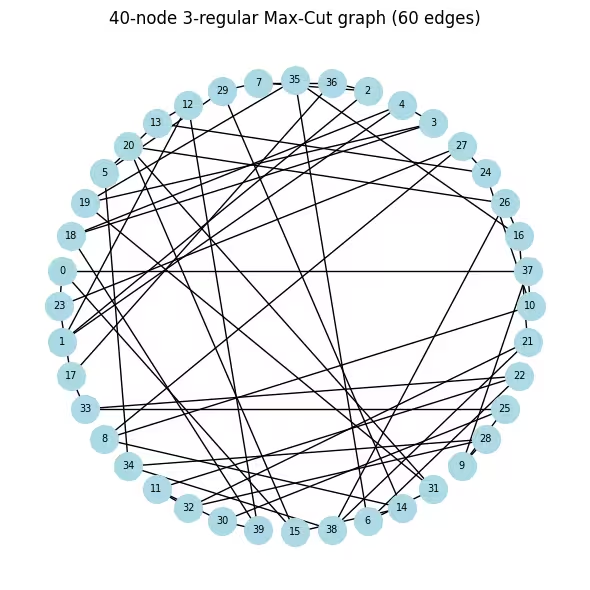
# A 3-regular graph (every node has exactly 3 neighbors) is a standard QAOA
N_LARGE = 40
G_large = nx.random_regular_graph(d=3, n=N_LARGE, seed=0)
edges_large = list(G_large.edges())
print(f"Graph: {N_LARGE} nodes, {len(edges_large)} edges (3-regular)")

# Visualize the graph so it is clear what problem we are solving before any
# quantum work. Nodes in a circular layout; each edge contributes +1 to the
# cut value when its endpoints land in different partitions.
pos_large = nx.circular_layout(G_large)
fig, ax = plt.subplots(figsize=(6, 6))
nx.draw(
    G_large,
    pos_large,
    with_labels=True,
    node_color="lightblue",
    node_size=400,
    font_size=7,
    ax=ax,
)
ax.set_title(f"40-node 3-regular Max-Cut graph ({len(edges_large)} edges)")
plt.tight_layout()
plt.show()

# Same Maxcut → OptimizationProblem → QUBO → Ising pipeline as the small example,
# applied to the 40-node graph.
prob_large = Maxcut(G_large).to_optimization_problem()
converter_large = OptimizationProblemToQubo()
qubo_large = converter_large.convert(prob_large)
cost_op_large, offset_large = to_ising(qubo_large)
n_qubits_large = cost_op_large.num_qubits
print(
    f"Cost operator: {n_qubits_large} qubits, {len(cost_op_large)} Pauli terms"
)

# ── Step 1b: QP relaxation (multi-start L-BFGS-B) ─────────────────────────
# Same multi-start approach as the small example. At 40 qubits the relaxed
# landscape has many more local minima, so 200 random starts are essential
# to find a low-energy warm-start point.
Q_large = qubo_large.objective.quadratic.to_array(symmetric=True)
mu_large = qubo_large.objective.linear.to_array()

def qp_obj_large(x):
    return x @ Q_large @ x + mu_large @ x + qubo_large.objective.constant

bounds_large = [(0.0, 1.0)] * n_qubits_large
rng_qp = np.random.default_rng(42)
best_val_large, c_star_large = np.inf, None

for _ in range(200):
    x0 = rng_qp.uniform(0.0, 1.0, n_qubits_large)
    res = minimize(qp_obj_large, x0, method="L-BFGS-B", bounds=bounds_large)
    if res.fun < best_val_large:
        best_val_large, c_star_large = res.fun, res.x

# Regularize and convert to rotation angles (same formula as small example)
epsilon_large = 0.25
c_clipped_large = np.clip(c_star_large, epsilon_large, 1 - epsilon_large)
thetas_large = 2 * np.arcsin(np.sqrt(c_clipped_large))
print(
    f"c* range: [{c_star_large.min():.3f}, {c_star_large.max():.3f}]  "
    f"theta range: [{thetas_large.min():.3f}, {thetas_large.max():.3f}] rad"
)

# Plot the distribution of c* values to see how much structure the relaxation
# extracted. Values near 0/1 mean confident assignments; values near 0.5 mean
# the classical solver was uncertain and quantum exploration is most needed there.
fig, ax = plt.subplots(figsize=(6, 3))
ax.hist(c_star_large, bins=20, color="steelblue", edgecolor="white")
ax.axvline(0.5, color="k", linestyle="--", label="Uniform prior (std QAOA)")
ax.set_xlabel(r"$c^*_i$")
ax.set_ylabel("Count")
ax.set_title(r"Distribution of warm-start values $c^*_i$ (40-node graph)")
ax.legend()
plt.tight_layout()
plt.show()

# ── Step 1c: Build WS-QAOA circuit ─────────────────────────────────────────
# Reuse build_ws_qaoa from the small-scale section unchanged; the helper
# scales automatically with n_qubits and the cost operator size.
p_large = 1
ws_qc_large, ws_gammas_large, ws_betas_large = build_ws_qaoa(
    cost_op_large, p_large, n_qubits_large, thetas_large
)
ws_qc_large.measure_all()

# ── Step 2: Transpile to hardware-native gates ──────────────────────────
# generate_preset_pass_manager compiles the abstract circuit to th
# gate set of the backend and inserts SWAP gates wherever the cost Hamiltonian
# couples qubits that are not directly connected on the processor.
pm = generate_preset_pass_manager(optimization_level=3, backend=backend)
ws_isa_large = pm.run(ws_qc_large)

ecr_count = ws_isa_large.count_ops().get("ecr", 0)
print(
    f"\nTranspiled circuit: 2Q depth={ws_isa_large.depth(lambda x: x.operation.num_qubits == 2)}"
)
ws_isa_large.draw("mpl", fold=-1)
Graph: 40 nodes, 60 edges (3-regular)
Cost operator: 40 qubits, 60 Pauli terms
c* range: [0.000, 1.000]  theta range: [1.047, 2.094] rad

Transpiled circuit: 2Q depth=86

# ── Classical baseline via simulated annealing ────────────────────
# Run SA before any hardware calls to get a strong classical reference cut
# value. SA is fast (seconds), needs no solver license, and reliably finds
# near-optimal solutions on 40-node graphs. We use sa_cut as the denominator
# for the approximation ratio instead of the looser QP upper bound.
#
# At each step we flip a random node and accept the move if it improves the
# cut, or with probability exp(delta/T) otherwise. Temperature T decays
# geometrically, allowing uphill moves early on to escape local minima.
def simulated_annealing_maxcut(
    G, seed=0, T0=2.0, T_min=1e-4, alpha=0.995, n_steps=100_000
):
    rng_sa = np.random.default_rng(seed)
    n = G.number_of_nodes()
    x = rng_sa.integers(0, 2, n)
    best_x = x.copy()
    best_cut = sum(1 for u, v in G.edges() if x[u] != x[v])
    T = T0
    for _ in range(n_steps):
        i = rng_sa.integers(0, n)
        delta = sum((-1 if x[i] != x[nb] else 1) for nb in G.neighbors(i))
        if delta > 0 or rng_sa.random() < np.exp(delta / T):
            x[i] ^= 1
            cut = sum(1 for u, v in G.edges() if x[u] != x[v])
            if cut > best_cut:
                best_cut, best_x = cut, x.copy()
        T = max(T * alpha, T_min)
    return best_x, best_cut

sa_solution, sa_cut = simulated_annealing_maxcut(G_large)
print(f"Simulated annealing cut value: {sa_cut}  (classical reference)")

# ── Step 3: Execution on hardware ───────────────────────────
# A Session reserves the backend so the COBYLA iterations and final sampling
# run back-to-back without re-queuing between jobs — important when the
# optimizer submits many short jobs sequentially. All jobs are tagged with
# "TUT_WSQAOA" for traceability in the IBM Quantum dashboard.
#
# EstimatorV2 with resilience_level=1 enables twirled readout error extinction
# (TREX), which corrects systematic measurement bit-flip errors without extra
# circuit overhead. 4096 shots per call balances estimation noise vs. job time.
estimator_options = EstimatorOptions()
estimator_options.resilience_level = 1
estimator_options.default_shots = 4096
estimator_options.environment.job_tags = ["TUT_WSQAOA"]

# Align the cost observable with the physical qubit layout chosen by the transpiler
cost_op_isa = cost_op_large.apply_layout(ws_isa_large.layout)
ws_param_order_isa = list(ws_isa_large.parameters)

ws_history_hw = []

with Session(backend=backend) as session:
    estimator_hw = Estimator(mode=session, options=estimator_options)

    def hw_cost_fn(params):
        bound = ws_isa_large.assign_parameters(
            dict(zip(ws_param_order_isa, params))
        )
        energy = (
            estimator_hw.run([(bound, cost_op_isa)]).result()[0].data.evs.real
        )
        ws_history_hw.append(float(energy))
        print(
            f"  iter {len(ws_history_hw):>3d}  <H_C> = {energy:.4f}", end="\r"
        )
        return float(energy)

    # Warm-start initialization: gamma=0 means the cost unitary is the identity on
    # the first call, so COBYLA immediately evaluates the warm-start state itself —
    # a much better starting signal than a random point.
    ws_params0_hw = np.concatenate(
        [np.zeros(p_large), np.full(p_large, np.pi / 4)]
    )

    ws_result_hw = minimize(
        hw_cost_fn,
        ws_params0_hw,
        method="COBYLA",
        options={"maxiter": 150, "rhobeg": 0.3},
    )
    print(
        f"\nOptimization complete: energy={ws_result_hw.fun:.4f}, "
        f"iterations={len(ws_history_hw)}"
    )

    # ── Step 3b: Sample the optimized circuit ──────────────────────────────────
    # Use 8192 shots for the final sample to get a reliable mode estimate.
    sampler_hw = Sampler(
        mode=session,
        options={"environment": {"job_tags": ["TUT_WSQAOA"]}},
    )
    ws_bound_hw = ws_isa_large.assign_parameters(
        dict(zip(ws_param_order_isa, ws_result_hw.x))
    )
    counts_hw = (
        sampler_hw.run([ws_bound_hw], shots=8192)
        .result()[0]
        .data.meas.get_counts()
    )

best_bs_hw = max(counts_hw, key=counts_hw.get)
best_count = counts_hw[best_bs_hw]
total_shots = sum(counts_hw.values())

# Decode: Qiskit returns bitstrings with qubit 0 at the rightmost position,
# so reversing the string maps character index i to variable x_i.
cut_val_hw, s0_hw, s1_hw = evaluate_cut(best_bs_hw[::-1], G_large)

# Compare against simulated annealing.
# A ratio >= 1.0 means WS-QAOA matched or beat the classical SA solution.
# A ratio close to 1.0 (e.g. > 0.95) shows the quantum result is competitive.
approx_ratio_hw = cut_val_hw / sa_cut
print(
    f"Most-probable bitstring frequency: {best_count}/{total_shots} "
    f"({100*best_count/total_shots:.1f}%)"
)
print(
    f"WS-QAOA cut: {cut_val_hw}  |  SA cut: {sa_cut}  "
    f"|  Approximation ratio vs SA: {approx_ratio_hw:.4f}"
)

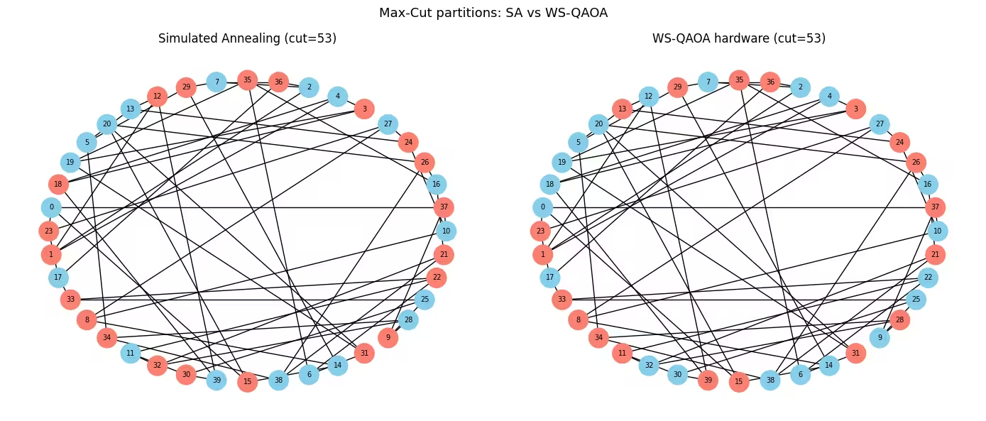
# Visualize both solutions side-by-side on the graph.
# Blue = partition S, orange = partition S-bar.
# Edges crossing between colors are the ones counted in the cut.
fig, axes = plt.subplots(1, 2, figsize=(14, 6))
for ax, assignment, cut, title in [
    (
        axes[0],
        list(sa_solution),
        sa_cut,
        f"Simulated Annealing (cut={sa_cut})",
    ),
    (
        axes[1],
        [int(b) for b in best_bs_hw[::-1]],
        cut_val_hw,
        f"WS-QAOA hardware (cut={cut_val_hw})",
    ),
]:
    colors = [
        "skyblue" if assignment[i] == 0 else "salmon" for i in G_large.nodes()
    ]
    nx.draw(
        G_large,
        pos_large,
        with_labels=True,
        node_color=colors,
        node_size=400,
        font_size=7,
        ax=ax,
    )
    ax.set_title(title)
plt.suptitle("Max-Cut partitions: SA vs WS-QAOA", fontsize=13)
plt.tight_layout()
plt.show()

# ── Step 4: Convergence plot and summary ──────────────────────────────────
# On real hardware the trace will be noisy (shot noise + gate errors), but the
# overall downward trend confirms that COBYLA is making progress despite noise.
fig, ax = plt.subplots(figsize=(7, 4))
ax.plot(ws_history_hw, color="tab:orange", label="WS-QAOA (hardware)")
ax.axhline(
    ws_result_hw.fun,
    color="tab:orange",
    linestyle=":",
    label=f"Final energy ({ws_result_hw.fun:.3f})",
)
ax.set_xlabel("Optimizer call")
ax.set_ylabel(r"$\langle H_C \rangle$")
ax.set_title(f"WS-QAOA convergence on {backend.name} (40 qubits, p=1)")
ax.legend()
plt.tight_layout()
plt.show()

print("\n=== Large Scale Summary ===")
print(f"{'Metric':<38} {'Value':>10}")
print("-" * 50)
print(f"{'Nodes / Edges':<38} {N_LARGE:>5} / {len(edges_large):<4}")
print(f"{'QAOA layers (p)':<38} {p_large:>10}")
print(f"{'Transpiled ECR gate count':<38} {ecr_count:>10}")
print(f"{'Transpiled circuit depth':<38} {ws_isa_large.depth():>10}")
print(f"{'Optimizer iterations':<38} {len(ws_history_hw):>10}")
print(f"{'WS-QAOA energy (hardware)':<38} {ws_result_hw.fun:>10.4f}")
print(f"{'Cut value':<38} {cut_val_hw:>10}")
print(f"{'Simulated annealing cut value':<38} {sa_cut:>10}")
print(f"{'Approximation ratio (vs SA)':<38} {approx_ratio_hw:>10.4f}")
Simulated annealing cut value: 53  (classical reference)
  iter  31  <H_C> = -12.4094
Optimization complete: energy=-13.0256, iterations=31
Most-probable bitstring frequency: 4/8192 (0.0%)
WS-QAOA cut: 53  |  SA cut: 53  |  Approximation ratio vs SA: 1.0000

=== Large Scale Summary ===
Metric                                      Value
--------------------------------------------------
Nodes / Edges                             40 / 60
QAOA layers (p)                                 1
Transpiled ECR gate count                       0
Transpiled circuit depth                      276
Optimizer iterations                           31
WS-QAOA energy (hardware)                -13.0256
Cut value                                      53
Simulated annealing cut value                  53
Approximation ratio (vs SA)                1.0000
צעדים הבאים
אם מצאת את העבודה הזאת מעניינת, ייתכן שתתעניין בחומר הבא:
- שכבות QAOA גבוהות יותר: הגדל את
pכדי לראות כיצד שני האלגוריתמים משתפרים עם יותר שכבות מעגל, ואם היתרון של WS-QAOA בעומק נמוך נשמר. - ממפה אופטימיזציה של תוסף Qiskit: חקור את התיעוד ונסה לדגמן בעיות קומבינטוריות שונות, או להשתמש בפותרים שונים עבור ההרפיה הרציפה.
מקורות
[1] D. J. Egger, J. Mareček, and S. Woerner, "Warm-starting quantum optimization," Quantum, vol. 5, p. 479, 2021. arXiv:2009.10095
[2] E. Farhi, J. Goldstone, and S. Gutmann, "A quantum approximate optimization algorithm," arXiv:1411.4028, 2014.