qubit, שערים ומעגלים קוונטיים

הערה

Kifumi Numata (19 Apr 2024)

לחץ/י כאן כדי להוריד את ה-PDF של ההרצאה המקורית. שים/י לב שחלק מקטעי הקוד עשויים להיות מיושנים, מכיוון שמדובר בתמונות סטטיות.

זמן QPU משוער להרצת הניסוי הזה הוא 5 שניות.

1. מבוא

ביטים, שערים ומעגלים הם אבני הבניין הבסיסיות של החישוב הקוונטי. תלמד/י חישוב קוונטי במודל המעגל באמצעות ביטים קוונטיים ושערים, וגם תסקור/י את הנושאים של סופרפוזיציה, מדידה וסבך קוונטי.

בשיעור זה תלמד/י:

• שערים של qubit בודד
• ספירת Bloch
• סופרפוזיציה
• מדידה
• שערים של שני qubit ומצב סבוך

בסוף ההרצאה תלמד/י על עומק המעגל, שהוא חיוני לחישוב קוונטי בסדר גודל של שימוש.

2. חישוב כדיאגרמה

כשמשתמשים ב-Qubit או בביטים, צריך לתפעל אותם כדי להפוך את הקלטים הקיימים לפלטים הרצויים. עבור התוכניות הפשוטות ביותר עם מספר קטן מאוד של ביטים, שימושי לייצג תהליך זה בדיאגרמה הידועה בשם דיאגרמת מעגל.

הדמות בפינה השמאלית התחתונה היא דוגמה למעגל קלאסי, ואילו הדמות בפינה הימנית התחתונה היא דוגמה למעגל קוונטי. בשני המקרים, הקלטים נמצאים בצד שמאל והפלטים בצד ימין, בעוד שהפעולות מיוצגות על ידי סמלים. הסמלים המשמשים לפעולות נקראים "שערים", בעיקר מסיבות היסטוריות.

3. שער קוונטי של qubit בודד

3.1 מצב קוונטי וספירת Bloch

מצב ה-Qubit מיוצג כסופרפוזיציה של $|0\rangle$ ו-$|1\rangle$. מצב קוונטי שרירותי מיוצג כ

$$|\psi\rangle =\alpha|0\rangle+ \beta|1\rangle$$

כאשר $\alpha$ ו-$\beta$ הם מספרים מרוכבים כך ש-$|\alpha|^2+|\beta|^2=1$.

$|0\rangle$ ו-$|1\rangle$ הם וקטורים במרחב הוקטורי המרוכב הדו-ממדי:

$$|0\rangle = \begin{pmatrix} 1 \\0 \end{pmatrix}, |1\rangle = \begin{pmatrix} 0\\1 \end{pmatrix}$$

לכן, מצב קוונטי שרירותי מיוצג גם כ

$$|\psi\rangle = \alpha\begin{pmatrix} 1 \\ 0 \end{pmatrix} + \beta\begin{pmatrix}0\\ 1 \end{pmatrix} = \begin{pmatrix} \alpha \\ \beta \end{pmatrix}$$

מכך ניתן לראות שמצב הביט הקוונטי הוא וקטור יחידה במרחב מכפלה פנימית מרוכב דו-ממדי עם בסיס אורתונורמלי של $|0\rangle$ ו-$|1\rangle$. הוא מנורמל ל-1.

$$\langle\psi|\psi\rangle = \begin{pmatrix} \alpha^* & \beta^* \end{pmatrix} \begin{pmatrix} \alpha \\ \beta \end{pmatrix} = 1$$

$|\psi\rangle =\begin{pmatrix} \alpha \\ \beta \end{pmatrix}$ נקרא גם וקטור המצב (statevector).

מצב קוונטי של qubit בודד מיוצג גם כ

$$|\psi\rangle =\cos\frac{\theta}{2}|0\rangle+e^{i\varphi}\sin\frac{\theta}{2}|1\rangle =\left( \begin{pmatrix} \cos\frac{\theta}{2}\\ e^{i\varphi}\sin\frac{\theta}{2} \end{pmatrix}\right)$$

כאשר $\theta$ ו-$\varphi$ הם הזוויות של ספירת Bloch בתרשים הבא.

בתאי הקוד הבאים, נבנה חישובים בסיסיים מחלקים בסיסיים ב-Qiskit. נבנה מעגל ריק ולאחר מכן נוסיף פעולות קוונטיות, נדון בשערים ונמחיש את ההשפעות שלהם תוך כדי. ניתן להריץ את התא ב-"Shift" + "Enter". ייבא/י את הספריות קודם.

# Added by doQumentation — required packages for this notebook
!pip install -q qiskit qiskit-aer qiskit-ibm-runtime

# Import the qiskit library
from qiskit import QuantumCircuit
from qiskit_aer import AerSimulator
from qiskit.quantum_info import Statevector
from qiskit.visualization import plot_bloch_multivector
from qiskit_ibm_runtime import Sampler
from qiskit.transpiler.preset_passmanagers import generate_preset_pass_manager
from qiskit.visualization import plot_histogram

הכנת ה-Circuit הקוונטי

נצור ונצייר Circuit של qubit בודד.

# Create the single-qubit quantum circuit
qc = QuantumCircuit(1)

# Draw the circuit
qc.draw("mpl")

שער X

שער ה-X הוא סיבוב של $\pi$ סביב ציר ה-$x$ של ספירת Bloch. החלת שער ה-X על $|0\rangle$ מניבה $|1\rangle$, והחלת שער ה-X על $|1\rangle$ מניבה $|0\rangle$, כך שזו פעולה דומה לשער NOT הקלאסי, והיא ידועה גם כהיפוך ביט. ייצוג המטריצה של שער ה-X מוצג למטה.

$$X = \begin{pmatrix} 0 & 1 \\ 1 & 0 \\ \end{pmatrix}$$

qc = QuantumCircuit(1)  # Prepare the single-qubit quantum circuit

# Apply a X gate to qubit 0
qc.x(0)

# Draw the circuit
qc.draw("mpl")

ב-IBM Quantum®, המצב ההתחלתי מוגדר כ-$|0\rangle$, כך שה-Circuit הקוונטי לעיל בייצוג מטריצה הוא

$$X|0\rangle= \begin{pmatrix} 0 & 1 \\ 1 & 0 \end{pmatrix} \begin{pmatrix} 1 \\ 0 \end{pmatrix} =\begin{pmatrix} 0 \\ 1 \end{pmatrix} = |1\rangle$$

עכשיו, בואו נריץ את ה-Circuit הזה באמצעות סימולטור statevector.

# See the statevector
out_vector = Statevector(qc)
print(out_vector)

# Draw a Bloch sphere
plot_bloch_multivector(out_vector)

Statevector([0.+0.j, 1.+0.j],
            dims=(2,))

הוקטור האנכי מוצג כוקטור שורה, עם מספרים מרוכבים (החלק הדמיוני מסומן ב-$j$).

שער H

שער Hadamard הוא סיבוב של $\pi$ סביב ציר הנמצא באמצע בין ציר ה-$x$ לציר ה-$z$ על ספירת Bloch. החלת שער ה-H על $|0\rangle$ יוצרת מצב סופרפוזיציה כגון $\frac{|0\rangle + |1\rangle}{\sqrt{2}}$. ייצוג המטריצה של שער ה-H מוצג למטה.

$$H = \frac{1}{\sqrt{2}}\begin{pmatrix} 1 & 1 \\ 1 & -1 \\ \end{pmatrix}$$

qc = QuantumCircuit(1)  # Create the single-qubit quantum circuit

# Apply an Hadamard gate to qubit 0
qc.h(0)

# Draw the circuit
qc.draw(output="mpl")

# See the statevector
out_vector = Statevector(qc)
print(out_vector)

# Draw a Bloch sphere
plot_bloch_multivector(out_vector)

Statevector([0.70710678+0.j, 0.70710678+0.j],
            dims=(2,))

זהו

$$H|0\rangle= \frac{1}{\sqrt{2}} \begin{pmatrix} 1 & 1 \\ 1 & -1 \end{pmatrix} \begin{pmatrix} 1 \\0 \end{pmatrix} =\frac{1}{\sqrt{2}}\begin{pmatrix} 1 \\ 1 \end{pmatrix} =\begin{pmatrix} 0.707 \\ 0.707 \end{pmatrix} =\frac{1}{\sqrt{2}}(|0\rangle+|1\rangle)$$

מצב הסופרפוזיציה הזה כל כך נפוץ וחשוב, עד שניתן לו סמל משלו:

$$|+\rangle \equiv \frac{1}{\sqrt{2}}(|0\rangle+|1\rangle).$$

על ידי החלת שער ה-$H$ על $|0\rangle$, יצרנו סופרפוזיציה של $|0\rangle$ ו-$|1\rangle$ שבה מדידה בבסיס החישובי (לאורך ציר z בתמונת ספירת Bloch) תיתן לך כל מצב בהסתברויות שוות.

מצב $|-\rangle$

אפשר שניחשת שיש מצב $|-\rangle$ מקביל:

$$|-\rangle \equiv \frac{|0\rangle -|1\rangle}{\sqrt{2}}.$$

כדי ליצור מצב זה, יש להחיל תחילה שער X כדי לקבל $|1\rangle$, ואז להחיל שער H.

qc = QuantumCircuit(1)  # Create the single-qubit quantum circuit

# Apply a X gate to qubit 0
qc.x(0)

# Apply an Hadamard gate to qubit 0
qc.h(0)

# draw the circuit
qc.draw(output="mpl")

# See the statevector
out_vector = Statevector(qc)
print(out_vector)

# Draw a Bloch sphere
plot_bloch_multivector(out_vector)

Statevector([ 0.70710678+0.j, -0.70710678+0.j],
            dims=(2,))

זהו

$$H|1\rangle= \frac{1}{\sqrt{2}} \begin{pmatrix} 1 & 1 \\\ 1 & -1 \end{pmatrix} \begin{pmatrix} 0 \\\ 1 \end{pmatrix} =\frac{1}{\sqrt{2}}\begin{pmatrix} 1 \\\ -1 \end{pmatrix} =\begin{pmatrix} 0.707 \\\ -0.707 \end{pmatrix} =\frac{1}{\sqrt{2}}(|0\rangle-|1\rangle) = |-\rangle$$

החלת שער ה-$H$ על $|1\rangle$ מניבה סופרפוזיציה שווה של $|0\rangle$ ו-$|1\rangle$, אך הסימן של $|1\rangle$ שלילי.

3.2 מצב קוונטי של qubit בודד ואבולוציה יוניטרית

הפעולות של כל ה-Gate-ים שראינו עד כה היו יוניטריות, כלומר ניתן לייצגן באמצעות אופרטור יוניטרי. במילים אחרות, מצב הפלט מתקבל על ידי פעולה על המצב ההתחלתי עם מטריצה יוניטרית:

$$|\psi^{'}\rangle = U|\psi\rangle$$

מטריצה יוניטרית היא מטריצה המקיימת

$$U^{\dagger}U =U U^{\dagger} = I.$$

מבחינת פעולת המחשב הקוונטי, נאמר שהחלת Gate קוונטי על ה-Qubit מפתחת את המצב הקוונטי. Gate-ים נפוצים של qubit בודד כוללים את הבאים.

Gate-י פאולי:

$$X = \begin{pmatrix} 0 & 1 \\ 1 & 0 \\ \end{pmatrix} = |0\rangle \langle 1|+|1\rangle \langle 0|$$ $$Y = \begin{pmatrix} 0 & -i \\ i & 0 \\ \end{pmatrix} = -i|0\rangle \langle 1|+i|1\rangle \langle 0|$$ $$Z = \begin{pmatrix} 1 & 0 \\ 0 & -1 \\ \end{pmatrix} = |0\rangle \langle 0|-|1\rangle \langle 1|$$

כאשר המכפלה החיצונית חושבה כך:

$$|0\rangle \langle 0|= \begin{bmatrix} 1 \\ 0 \end{bmatrix} \begin{bmatrix} 1 & 0 \end{bmatrix} =\begin{bmatrix} 1 & 0 \\ 0 & 0 \\ \end{bmatrix}, \quad |1\rangle \langle 0|= \begin{bmatrix} 0 \\ 1 \end{bmatrix} \begin{bmatrix} 1 & 0 \end{bmatrix} =\begin{bmatrix} 0 & 0 \\ 1 & 0 \\ \end{bmatrix}, \quad$$ $$|0\rangle \langle 1|= \begin{bmatrix} 1 \\ 0 \end{bmatrix} \begin{bmatrix} 0 & 1 \end{bmatrix} =\begin{bmatrix} 0 & 1 \\ 0 & 0 \\ \end{bmatrix}, \quad |1\rangle \langle 1|= \begin{bmatrix} 0 \\ 1 \end{bmatrix} \begin{bmatrix} 0 & 1 \end{bmatrix} =\begin{bmatrix} 0 & 0 \\ 0 & 1 \\ \end{bmatrix}, \quad$$

Gate-ים נוספים נפוצים של qubit בודד:

$$H= \frac{1}{\sqrt{2}}\begin{bmatrix} 1 & 1 \\ 1 & -1 \\ \end{bmatrix},\quad S = \begin{bmatrix} 1 & 0 \\ 0 & i \\ \end{bmatrix}, \quad T = \begin{bmatrix} 1 & 0 \\ 0 & exp(i\pi/4) \\ \end{bmatrix}$$ $$R_x(\theta) = e^{-i\theta X/2} = cos\frac{\theta}{2}I - i sin \frac{\theta}{2}X = \begin{bmatrix} cos\frac{\theta}{2} & -i sin \frac{\theta}{2} \\ -i sin \frac{\theta}{2} & cos\frac{\theta}{2} \\ \end{bmatrix}$$ $$R_y(\theta) = e^{-i\theta Y/2} = cos\frac{\theta}{2}I - i sin \frac{\theta}{2}Y = \begin{bmatrix} cos\frac{\theta}{2} & - sin \frac{\theta}{2} \\ sin \frac{\theta}{2} & cos\frac{\theta}{2} \\ \end{bmatrix}$$ $$R_z(\theta) = e^{-i\theta Z/2} = cos\frac{\theta}{2}I - i sin \frac{\theta}{2}Z = \begin{bmatrix} e^{-i\theta /2} & 0 \\ 0 & e^{i\theta /2} \\ \end{bmatrix}$$

המשמעות והשימוש בהם מתוארים בפירוט רב יותר בקורס יסודות המידע הקוונטי.

תרגיל 1

השתמש ב-Qiskit כדי ליצור Circuit-ים קוונטיים שמכינים את המצבים המתוארים להלן. לאחר מכן הרץ כל Circuit באמצעות סימולטור ה-statevector והצג את המצב המתקבל על כדור בלוך. כבונוס, נסה לנחש מה יהיה המצב הסופי על סמך אינטואיציה לגבי ה-Gate-ים והסיבובים בכדור בלוך.

(1) $XX|0\rangle$

(2) $HH|0\rangle$

(3) $HZH|0\rangle$

טיפים: ניתן להשתמש ב-Z Gate באופן הבא:

qc.z(0)

פתרון:

### (1) XX|0> ###

# Create the single-qubit quantum circuit
qc = QuantumCircuit(1)  ##your code goes here##

# Add a X gate to qubit 0
qc.x(0)  ##your code goes here##

# Add a X gate to qubit 0
qc.x(0)  ##your code goes here##

# Draw a circuit
qc.draw(output="mpl")

# See the statevector
out_vector = Statevector(qc)
print(out_vector)

# Draw a Bloch sphere
plot_bloch_multivector(out_vector)

Statevector([1.+0.j, 0.+0.j],
            dims=(2,))

### (2) HH|0> ###
##your code goes here##
qc = QuantumCircuit(1)
qc.h(0)
qc.h(0)
qc.draw("mpl")

# See the statevector
out_vector = Statevector(qc)
print(out_vector)

# Draw a Bloch sphere
plot_bloch_multivector(out_vector)

Statevector([1.+0.j, 0.+0.j],
            dims=(2,))

### (3) HZH|0> ###
##your code goes here##
qc = QuantumCircuit(1)
qc.h(0)
qc.z(0)
qc.h(0)
qc.draw("mpl")

# See the statevector
out_vector = Statevector(qc)
print(out_vector)

# Draw a Bloch sphere
plot_bloch_multivector(out_vector)

Statevector([0.+0.j, 1.+0.j],
            dims=(2,))

3.3 מדידה

מדידה היא נושא תיאורטי מורכב מאוד. אבל במונחים מעשיים, ביצוע מדידה לאורך $z$ (כפי שכל מחשבי הקוונטום של IBM® עושים) פשוט כופה על מצב ה-Qubit $\alpha|0\rangle+\beta|1\rangle \quad (s.t.|\alpha|^2+|\beta|^2=1)$ לקפוץ למצב $|0\rangle$ או $|1\rangle$, ואנחנו צופים בתוצאה.

• $|\alpha|^2$ הוא ההסתברות שנקבל $|0\rangle$ בעת המדידה.
• $|\beta|^2$ הוא ההסתברות שנקבל $|1\rangle$ בעת המדידה.

לכן, $\alpha$ ו-$\beta$ נקראים משרעות הסתברות. (ראה "כלל בורן")

לדוגמה, ל-$\frac{\sqrt{2}}{2}|0\rangle+\frac{\sqrt{2}}{2}|1\rangle$ יש הסתברות שווה להפוך ל-$|0\rangle$ או $|1\rangle$ בעת המדידה. ל-$\frac{\sqrt{3}}{2}|0\rangle-\frac{1}{2}i|1\rangle$ יש סיכוי של 75% להפוך ל-$|0\rangle$.

סימולטור Qiskit Aer

עכשיו, בוא נמדוד Circuit שמכין את הסופרפוזיציה בהסתברות שווה שהוזכרה למעלה. עלינו להוסיף Gate-י מדידה, שכן סימולטור Qiskit Aer מדמה חומרה קוונטית אידיאלית (ללא רעש) כברירת מחדל. הערה: הסימולטור Aer יכול גם להחיל מודל רעש המבוסס על מחשב קוונטי אמיתי. נחזור למודלי רעש מאוחר יותר.

# Create a new circuit with one qubits (first argument) and one classical bits (second argument)
qc = QuantumCircuit(1, 1)
qc.h(0)
qc.measure(0, 0)  # Add the measurement gate

qc.draw(output="mpl")

עכשיו אנחנו מוכנים להריץ את ה-Circuit שלנו על סימולטור Aer. בדוגמה זו, נשתמש ב-shots=1024 כברירת מחדל, כלומר נמדוד 1024 פעמים. לאחר מכן נציג את הספירות האלו בהיסטוגרמה.

# Run the circuit on a simulator to get the results
# Define backend
backend = AerSimulator()

# Transpile to backend
pm = generate_preset_pass_manager(backend=backend, optimization_level=1)
isa_qc = pm.run(qc)

# Run the job
sampler = Sampler(mode=backend)
job = sampler.run([isa_qc])
result = job.result()

# Print the results
counts = result[0].data.c.get_counts()
print(counts)

# Plot the counts in a histogram
plot_histogram(counts)

{'0': 521, '1': 503}

אנחנו רואים ש-0 ו-1 נמדדו עם הסתברות של כמעט 50% כל אחד. למרות שרעש לא הדמינו כאן, המצבים עדיין הסתברותיים. לכן, בעוד שאנחנו מצפים לפיזור של 50-50 בערך, נדיר שנמצא בדיוק כזה. בדיוק כמו שהטלת מטבע 100 פעמים נדיר שתניב בדיוק 50 מופעים של כל צד.

4. Gate קוונטי רב-Qubit ושזירה

4.1 מעגל קוונטי רב-Qubit

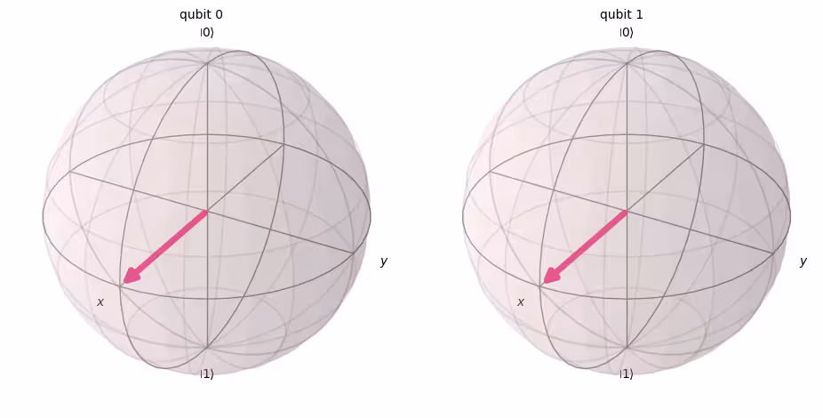
אפשר ליצור מעגל קוונטי של שני Qubitים עם הקוד הבא. נחיל Gate מסוג H על כל qubit.

# Create the two qubits quantum circuit
qc = QuantumCircuit(2)

# Apply an H gate to qubit 0
qc.h(0)

# Apply an H gate to qubit 1
qc.h(1)

# Draw the circuit
qc.draw(output="mpl")

# See the statevector
out_vector = Statevector(qc)
print(out_vector)

Statevector([0.5+0.j, 0.5+0.j, 0.5+0.j, 0.5+0.j],
            dims=(2, 2))

הערה: סדר הביטים ב-Qiskit

Qiskit משתמש בסימון Little Endian לסדר Qubitים וביטים, כלומר qubit 0 הוא הביט הימני ביותר במחרוזות הביטים. לדוגמה: $|01\rangle$ פירושו ש-q0 נמצא במצב $|1\rangle$ וש-q1 נמצא במצב $|0\rangle$. חשוב לשים לב לכך, כי חלק מהספרות בחישוב קוונטי משתמשות בסימון Big Endian (qubit 0 הוא הביט השמאלי ביותר), וכך גם חלק ניכר מהספרות של מכניקת הקוונטים.

דבר נוסף שראוי לשים לב אליו הוא שכאשר מציגים מעגל קוונטי, $|q_0\rangle$ ממוקם תמיד בחלק העליון של המעגל. עם זאת בחשבון, המצב הקוונטי של המעגל לעיל ניתן לכתיבה כמכפלת טנסור של מצבים קוונטיים של qubit בודד.

$|q1\rangle \otimes|q0\rangle = (a|0\rangle+b|1\rangle) \otimes (c|0\rangle+d|1\rangle)$

$= ac|0\rangle|0\rangle+ad|0\rangle|1\rangle+bc|1\rangle|0\rangle+bd|1\rangle|1\rangle$

$= ac|00\rangle+ad|01\rangle+bc|10\rangle+bd|11\rangle$

( $|ac|^2+ |ad|^2+ |bc|^2+ |bd|^2=1$ )

המצב ההתחלתי של Qiskit הוא $|0\rangle|0\rangle=|00\rangle$, ולכן כשמחילים $H$ על כל qubit, המצב משתנה לסופרפוזיציה שווה.

$H|0\rangle \otimes H|0\rangle=\frac{1}{\sqrt{2}}(|0\rangle+|1\rangle) \otimes \frac{1}{\sqrt{2}}(|0\rangle+|1\rangle) = \frac{1}{2}(|00\rangle+|01\rangle+|10\rangle+|11\rangle)$

$$=\frac{1}{2}\left( \begin{pmatrix} 1 \\ 1 \end{pmatrix} \otimes \begin{pmatrix} 1 \\ 1 \end{pmatrix}\right) = \frac{1}{2}\begin{pmatrix} 1 \\ 1 \\ 1 \\ 1 \end{pmatrix}=\frac{1}{2}\left(\begin{pmatrix} 1 \\ 0 \\ 0 \\ 0 \end{pmatrix}+\begin{pmatrix} 0 \\ 1 \\ 0 \\ 0 \end{pmatrix}+\begin{pmatrix} 0 \\ 0 \\ 1 \\ 0 \end{pmatrix}+\begin{pmatrix} 0 \\ 0 \\ 0 \\ 1 \end{pmatrix}\right)$$

כלל המדידה זהה למקרה של qubit בודד — הסתברות למדידת $|00\rangle$ היא $|ac|^2$.

# Draw a Bloch sphere
plot_bloch_multivector(out_vector)

עכשיו בואו נמדוד את המעגל הזה.

# Create a new circuit with two qubits (first argument) and two classical bits (second argument)
qc = QuantumCircuit(2, 2)

# Apply the gates
qc.h(0)
qc.h(1)

# Add the measurement gates
qc.measure(0, 0)  # Measure qubit 0 and save the result in bit 0
qc.measure(1, 1)  # Measure qubit 1 and save the result in bit 1

# Draw the circuit
qc.draw(output="mpl")

עכשיו נשתמש שוב בסימולטור Aer כדי לאמת בצורה ניסויית שההסתברויות היחסיות של כל מצבי הפלט האפשריים אכן שווות בערך.

# Run the circuit on a simulator to get the results
# Define backend
backend = AerSimulator()

# Transpile to backend
pm = generate_preset_pass_manager(backend=backend, optimization_level=1)
isa_qc = pm.run(qc)

# Run the job
sampler = Sampler(mode=backend)
job = sampler.run([isa_qc])
result = job.result()

# Print the results
counts = result[0].data.c.get_counts()
print(counts)

# Plot the counts in a histogram
plot_histogram(counts)

{'10': 262, '01': 246, '00': 265, '11': 251}

כצפוי, המצבים $|00\rangle$, $|01\rangle$, $|10\rangle$, $|11\rangle$ נמדדו כל אחד בערך ב-25%.

4.2 Gateים קוונטיים רב-Qubit

CNOT gate

Gate מסוג CNOT (שנקרא גם "controlled NOT" או CX) הוא Gate של שני Qubitים, כלומר פעולתו מערבת שני Qubitים בו-זמנית: Qubit הבקרה (control) ו-Qubit המטרה (target). ה-CNOT הופך את qubit המטרה רק כאשר qubit הבקרה נמצא במצב $|1\rangle$.

קלט (target,control)	פלט (target,control)
00	00
01	11
10	10
11	01

בואו נדמה תחילה את פעולת ה-Gate הדו-Qubit הזה כאשר q0 וגם q1 נמצאים במצב $|0\rangle$, ונקבל את וקטור המצב של הפלט. התחביר של Qiskit הוא qc.cx(control qubit, target qubit).

# Create a circuit with two quantum registers and two classical registers
qc = QuantumCircuit(2, 2)

# Apply the CNOT (cx) gate to a |00> state.
qc.cx(0, 1)  # Here the control is set to q0 and the target is set to q1.

# Draw the circuit
qc.draw(output="mpl")

# See the statevector
out_vector = Statevector(qc)
print(out_vector)

Statevector([1.+0.j, 0.+0.j, 0.+0.j, 0.+0.j],
            dims=(2, 2))

כצפוי, הפעלת CNOT gate על $|00\rangle$ לא שינתה את המצב, מכיוון ש-Qubit הבקרה היה במצב $|0\rangle$. נחזור לפעולת ה-CNOT שלנו. הפעם נחיל CNOT gate על $|01\rangle$ ונראה מה קורה.

qc = QuantumCircuit(2, 2)

# q0=1, q1=0
qc.x(0)  # Apply a X gate to initialize q0 to 1
qc.cx(0, 1)  # Set the control bit to q0 and the target bit to q1.

# Draw the circuit
qc.draw(output="mpl")

# See the statevector
out_vector = Statevector(qc)
print(out_vector)

Statevector([0.+0.j, 0.+0.j, 0.+0.j, 1.+0.j],
            dims=(2, 2))

על ידי הפעלת CNOT gate, המצב $|01\rangle$ הפך עכשיו ל-$|11\rangle$.

בואו נאמת את התוצאות האלה על ידי הרצת המעגל על סימולטור.

# Add measurements
qc.measure(0, 0)
qc.measure(1, 1)

# Draw the circuit
qc.draw(output="mpl")

# Run the circuit on a simulator to get the results
# Define backend
backend = AerSimulator()

# Transpile to backend
pm = generate_preset_pass_manager(backend=backend, optimization_level=1)
isa_qc = pm.run(qc)

# Run the job
sampler = Sampler(backend)
job = sampler.run([isa_qc])
result = job.result()

# Print the results
counts = result[0].data.c.get_counts()
print(counts)

# Plot the counts in a histogram
plot_histogram(counts)

{'11': 1024}

התוצאות אמורות להראות לך ש-$|11\rangle$ נמדד בהסתברות של 100%.

4.3 שזירה קוונטית והרצה על מחשב קוונטי אמיתי

בואו נתחיל בהצגת מצב שזור ספציפי שחשוב במיוחד בחישוב קוונטי, ואז נגדיר את המונח "שזור":

$$\frac{1}{\sqrt{2}}|00\rangle + \frac{1}{\sqrt{2}}|11\rangle$$

ומצב זה נקרא מצב Bell.

מצב שזור הוא מצב $|\psi_{AB}\rangle$ המורכב ממצבים קוונטיים $|\psi_A\rangle$ ו-$|\psi_B\rangle$ שאינו יכול להיות מיוצג כמכפלת טנסור של מצבים קוונטיים נפרדים.

אם ל-$|\psi_{AB}\rangle$ הבא יש שני מצבים $|\psi\rangle_A$ ו-$|\psi\rangle_B$:

$$|\psi_{AB}\rangle = \frac{1}{\sqrt{2}}(|00\rangle +|11\rangle) = \frac{1}{\sqrt{2}}(|0\rangle_A|0\rangle_B +|1\rangle_A|1\rangle_B)$$ $$|\psi\rangle_A = a_0|0\rangle+a_1|1\rangle$$ $$|\psi\rangle_B = b_0|0\rangle+b_1|1\rangle$$

אז מכפלת הטנסור של שני המצבים הללו היא

$$|\psi\rangle _A\otimes |\psi\rangle _B = a_0 b_0|00\rangle+a_0 b_1|01\rangle+a_1 b_0|10\rangle+a_1 b_1|11\rangle$$

אבל אין מקדמים $a_0, a_1, b_0,$ ו-$b_1$ שיכולים לקיים את שתי המשוואות הללו. לכן, $|\psi_{AB}\rangle$ אינו מיוצג כמכפלת טנסור של מצבים קוונטיים נפרדים $|\psi\rangle_A$ ו-$|\psi\rangle_B$, וזה אומר ש-$|\psi_{AB}\rangle = \frac{1}{\sqrt{2}}(|00\rangle +|11\rangle)$ הוא מצב שזור.

בואו ניצור את מצב Bell ונריץ אותו על מחשב קוונטי אמיתי. נפעל לפי ארבעת השלבים לכתיבת תוכנית קוונטית, הנקראים Qiskit patterns:

1. Map problem to quantum circuits and operators
2. Optimize for target hardware
3. Execute on target hardware
4. Post-process the results

שלב 1. מיפוי הבעיה למעגלים קוונטיים ואופרטורים

בתוכנית קוונטית, מעגלים קוונטיים הם הפורמט הטבעי לייצוג הוראות קוונטיות. כשיוצרים מעגל, בדרך כלל יוצרים אובייקט QuantumCircuit חדש ולאחר מכן מוסיפים לו הוראות ברצף.

תא הקוד הבא יוצר מעגל שמייצר מצב Bell — המצב השזור הדו-Qubit הספציפי שהוצג למעלה.

qc = QuantumCircuit(2, 2)

qc.h(0)
qc.cx(0, 1)

qc.measure(0, 0)
qc.measure(1, 1)

qc.draw("mpl")

שלב 2. אופטימיזציה לחומרת היעד

Qiskit ממיר מעגלים מופשטים למעגלי QISA (Quantum Instruction Set Architecture) שמכבדים את מגבלות חומרת היעד ומייטב את ביצועי המעגל. לכן, לפני האופטימיזציה נגדיר את חומרת היעד. אם אין לך את qiskit-ibm-runtime, תצטרך להתקין אותה תחילה. למידע נוסף על Qiskit Runtime, ראה בחומר עזר של ה-API.

# Install
# !pip install qiskit-ibm-runtime

נגדיר את חומרת היעד.

from qiskit_ibm_runtime import QiskitRuntimeService

service = QiskitRuntimeService()
service.backends()

# You can specify the device
# backend = service.backend('ibm_kingston')

# You can also identify the least busy device
backend = service.least_busy(operational=True)
print("The least busy device is ", backend)

טרנספילציה של המעגל היא תהליך מורכב בפני עצמו. בקצרה, התהליך הזה כותב מחדש את המעגל לכזה שלוגית שקול לו, תוך שימוש ב"Gateים הטבעיים" (Gateים שמחשב קוונטי מסוים יכול לבצע) וממפה את ה-Qubitים במעגל שלך ל-Qubitים אמיתיים אופטימליים על המחשב הקוונטי המיועד. לפרטים נוספים על טרנספילציה, ראה את התיעוד.

# Transpile the circuit into basis gates executable on the hardware
pm = generate_preset_pass_manager(backend=backend, optimization_level=1)
target_circuit = pm.run(qc)

target_circuit.draw("mpl", idle_wires=False)

ניתן לראות שבמהלך הטרנספילציה המעגל נכתב מחדש עם Gateים חדשים. למידע נוסף, ראה בתיעוד של ECRGate.

שלב 3. הרצת מעגל היעד

עכשיו נריץ את מעגל היעד על המכשיר האמיתי.

sampler = Sampler(backend)
job_real = sampler.run([target_circuit])

job_id = job_real.job_id()
print("job id:", job_id)

הרצה על המכשיר האמיתי עשויה לדרוש המתנה בתור, מכיוון שמחשבים קוונטיים הם משאבים יקרי ערך ומבוקשים מאוד. ה-job_id משמש לבדיקת סטטוס ההרצה ותוצאות ה-Job בהמשך.

# Check the job status (replace the job id below with your own)
job_real.status(job_id)

אפשר גם לבדוק את סטטוס ה-Job מלוח הבקרה של IBM Quantum שלך: https://quantum.cloud.ibm.com/workloads

# If the Notebook session got disconnected you can also check your job status
# by running the following code
from qiskit_ibm_runtime import QiskitRuntimeService

service = QiskitRuntimeService()
job_real = service.job(job_id)  # Input your job-id between the quotations
job_real.status()

# Execute after job has successfully run
result_real = job_real.result()
print(result_real[0].data.c.get_counts())

שלב 4. עיבוד לאחר של התוצאות

לבסוף, עלינו לעבד את התוצאות שלנו כדי ליצור פלטים בפורמט הצפוי, כמו ערכים או גרפים.

plot_histogram(result_real[0].data.c.get_counts())

כפי שניתן לראות, $|00\rangle$ ו-$|11\rangle$ הם המצבים הנצפים בתדירות הגבוהה ביותר. ישנן מספר תוצאות נוספות מעבר לנתונים הצפויים, והן נובעות מרעש ודה-קוהרנטיות של Qubitים. נלמד עוד על שגיאות ורעש במחשבים קוונטיים בשיעורים המאוחרים יותר של קורס זה.

4.4 מצב GHZ

הרעיון של שזירה יכול להתרחב למערכות של יותר משני Qubitים. מצב GHZ (מצב גרינברגר-הורן-זילינגר) הוא מצב שזור מקסימלי של שלושה Qubitים או יותר. מצב ה-GHZ עבור שלושה Qubitים מוגדר כ:

$$\frac{1}{\sqrt 2}(|000\rangle + |111\rangle)$$

אפשר ליצור אותו עם ה-Circuit הקוונטי הבא.

qc = QuantumCircuit(3, 3)

qc.h(0)
qc.cx(0, 1)
qc.cx(1, 2)

qc.measure(0, 0)
qc.measure(1, 1)
qc.measure(2, 2)

qc.draw("mpl")

"העומק" של Circuit קוונטי הוא מדד שימושי ונפוץ לתיאור Circuitים קוונטיים. עוקבים אחר מסלול דרך ה-Circuit הקוונטי, נעים משמאל לימין, ומחליפים Qubitים רק כשהם מחוברים ע"י Gate רב-Qubit. סופרים את מספר ה-Gateים לאורך אותו מסלול. המספר המרבי של Gateים בכל מסלול כזה דרך Circuit הוא העומק. במחשבים קוונטיים רועשים מודרניים, Circuitים בעלי עומק נמוך מניבים פחות שגיאות וסביר שיחזירו תוצאות טובות. Circuitים עמוקים מאוד — לא.

בעזרת QuantumCircuit.depth(), אפשר לבדוק את עומק ה-Circuit הקוונטי שלנו. עומקו של ה-Circuit שלמעלה הוא 4. ל-Qubit העליון יש רק שלושה Gateים כולל המדידה. אך יש מסלול מה-Qubit העליון למטה לכל אחד מ-Qubit 1 או qubit 2 שכולל Gate CNOT נוסף.

qc.depth()

4

תרגיל 2

מצב ה-GHZ של מערכת 8 Qubitים הוא

$$\frac{1}{\sqrt 2}(|00000000\rangle + |11111111\rangle)$$

כתבו קוד להכנת מצב זה עם ה-Circuit הרדוד ביותר האפשרי. עומקו של ה-Circuit הקוונטי הרדוד ביותר הוא 5, כולל Gateי המדידה.

פתרון:

# Step 1
qc = QuantumCircuit(8, 8)

##your code goes here##
qc.h(0)
qc.cx(0, 4)
qc.cx(4, 6)
qc.cx(6, 7)

qc.cx(4, 5)

qc.cx(0, 2)
qc.cx(2, 3)

qc.cx(0, 1)
qc.barrier()  # for visual separation

# measure
for i in range(8):
    qc.measure(i, i)

qc.draw("mpl")
# print(qc.depth())

print(qc.depth())

5

from qiskit.visualization import plot_histogram
# Step 2
# For this exercise, the circuit and operators are simple, so no optimizations are needed.

# Step 3
# Run the circuit on a simulator to get the results
backend = AerSimulator()

pm = generate_preset_pass_manager(backend=backend, optimization_level=1)
isa_qc = pm.run(qc)

sampler = Sampler(mode=backend)
job = sampler.run([isa_qc], shots=1024)
result = job.result()

counts = result[0].data.c.get_counts()
print(counts)

# Step 4
# Plot the counts in a histogram

plot_histogram(counts)

{'11111111': 535, '00000000': 489}

5. סיכום

למדתם חישוב קוונטי עם מודל ה-Circuit תוך שימוש ב-Qubitים וב-Gateים קוונטיים, וסקרתם סופרפוזיציה, מדידה ושזירה. כמו כן, למדתם את השיטה להרצת ה-Circuit הקוונטי על המכשיר הקוונטי האמיתי.

בתרגיל הסופי ליצירת Circuit GHZ, ניסיתם להפחית את עומק ה-Circuit, שהוא גורם חשוב להשגת פתרון בסקאלת שימושיות במחשב קוונטי רועש. בשיעורים הבאים בקורס זה תלמדו על רעש ועל שיטות להפחתת שגיאות בפירוט. בשיעור זה, כהקדמה, שקלנו הפחתת עומק ה-Circuit במכשיר אידיאלי, אך במציאות יש להתחשב במגבלות של מכשיר אמיתי, כגון קישוריות Qubitים. תלמדו עוד על כך בשיעורים הבאים בקורס זה.

# See the version of Qiskit
import qiskit

qiskit.__version__

'2.0.2'