Quantum noise and error mitigation

הערה

Toshinari Itoko (28 יוני 2024)

הורד את קובץ ה-PDF של ההרצאה המקורית. שים לב שחלק מקטעי הקוד עשויים להיות מיושנים מכיוון שאלה תמונות סטטיות.

זמן QPU משוער להרצת הניסוי הזה הוא 1 דקה ו-40 שניות.

1. מבוא

לאורך השיעור הזה נבחן רעש וכיצד ניתן להפחית אותו במחשבים קוונטיים. נתחיל בבחינת השפעות הרעש באמצעות סימולטור שיכול לדמות רעש בכמה דרכים, כולל שימוש בפרופילי רעש ממחשבים קוונטיים אמיתיים. לאחר מכן נעבור למחשבים קוונטיים אמיתיים, שבהם הרעש הוא מובנה. נבחן את השפעות הפחתת השגיאות, כולל שילובים של דברים כמו אקסטרפולציית אפס-רעש (ZNE) וסיבוב Gate.

נתחיל בטעינת כמה חבילות.

# Added by doQumentation — required packages for this notebook
!pip install -q matplotlib qiskit qiskit-aer qiskit-ibm-runtime

# !pip install qiskit qiskit_aer qiskit_ibm_runtime
# !pip install jupyter
# !pip install matplotlib pylatexenc

import qiskit

qiskit.__version__

'2.0.2'

import qiskit_aer

qiskit_aer.__version__

'0.17.1'

import qiskit_ibm_runtime

qiskit_ibm_runtime.__version__

'0.40.1'

2. סימולציה רועשת ללא הפחתת שגיאות

Qiskit Aer הוא סימולטור קלאסי לחישוב קוונטי. הוא יכול לדמות לא רק הרצה אידיאלית אלא גם הרצה רועשת של Circuit קוונטי. מחברת זו ממחישה כיצד להריץ סימולציה רועשת באמצעות Qiskit Aer:

1. בנה מודל רעש
2. בנה Sampler רועש (סימולטור) עם מודל הרעש
3. הרץ Circuit קוונטי על ה-Sampler הרועש

noise_model = NoiseModel()
...
noisy_sampler = Sampler(options={"backend_options": {"noise_model": noise_model}})
job = noisy_sampler.run([circuit])

2.1 בנה Circuit בדיקה

אנחנו בוחנים Circuit של Qubit בודד לצורך משחק שפשוט חוזר על Gate ה-X d פעמים (d=0 ... 100) ומודד את הנצפה Z.

from qiskit.circuit import QuantumCircuit

MAX_DEPTH = 100
circuits = []
for d in range(MAX_DEPTH + 1):
    circ = QuantumCircuit(1)
    for _ in range(d):
        circ.x(0)
        circ.barrier(0)
    circ.measure_all()
    circuits.append(circ)

display(circuits[3].draw(output="mpl"))

from qiskit.quantum_info import SparsePauliOp

obs = SparsePauliOp.from_list([("Z", 1.0)])
obs

SparsePauliOp(['Z'],
              coeffs=[1.+0.j])

2.2 בנה מודל רעש

כדי לבצע סימולציה רועשת, אנחנו צריכים לציין NoiseModel. נראה כיצד לבנות NoiseModel בסעיף זה. קודם כל צריך להגדיר שגיאות קוונטיות (או שגיאות קריאה) להוספה למודל הרעש.

from qiskit_aer.noise.errors import (
    coherent_unitary_error,
    amplitude_damping_error,
    ReadoutError,
)
from qiskit.circuit.library import RXGate

# Coherent (unitary) error: Over X-rotation error
# https://qiskit.github.io/qiskit-aer/stubs/qiskit_aer.noise.coherent_unitary_error.html#qiskit_aer.noise.coherent_unitary_error
OVER_ROTATION_ANGLE = 0.05
coherent_error = coherent_unitary_error(RXGate(OVER_ROTATION_ANGLE).to_matrix())

# Incoherent error: Amplitude dumping error
# https://qiskit.github.io/qiskit-aer/stubs/qiskit_aer.noise.amplitude_damping_error.html#qiskit_aer.noise.amplitude_damping_error
AMPLITUDE_DAMPING_PARAM = 0.02  # in [0, 1] (0: no error)
incoherent_error = amplitude_damping_error(AMPLITUDE_DAMPING_PARAM)

# Readout (measurement) error: Readout error
# https://qiskit.github.io/qiskit-aer/stubs/qiskit_aer.noise.ReadoutError.html#qiskit_aer.noise.ReadoutError
PREP0_MEAS1 = 0.03  # P(1|0): Probability of preparing 0 and measuring 1
PREP1_MEAS0 = 0.08  # P(0|1): Probability of preparing 1 and measuring 0
readout_error = ReadoutError(
    [[1 - PREP0_MEAS1, PREP0_MEAS1], [PREP1_MEAS0, 1 - PREP1_MEAS0]]
)

from qiskit_aer.noise import NoiseModel

noise_model = NoiseModel()
noise_model.add_quantum_error(coherent_error.compose(incoherent_error), "x", (0,))
noise_model.add_readout_error(readout_error, (0,))

2.3 בנה Sampler רועש עם מודל הרעש

from qiskit_aer.primitives import SamplerV2 as Sampler

noisy_sampler = Sampler(options={"backend_options": {"noise_model": noise_model}})

2.4 הרץ Circuit קוונטי על ה-Sampler הרועש

job = noisy_sampler.run(circuits, shots=400)

result = job.result()

result[0].data.meas.get_counts()

{'0': 389, '1': 11}

2.5 הצג תוצאות

import matplotlib.pyplot as plt

plt.title("Noisy simulation")
ds = list(range(MAX_DEPTH + 1))
plt.plot(
    ds,
    [result[d].data.meas.expectation_values(["Z"]) for d in ds],
    color="gray",
    linestyle="-",
)
plt.scatter(ds, [result[d].data.meas.expectation_values(["Z"]) for d in ds], marker="o")
plt.hlines(0, xmin=0, xmax=MAX_DEPTH, colors="black")
plt.ylim(-1, 1)
plt.xlabel("Circuit depth")
plt.ylabel("Measured <Z>")
plt.show()

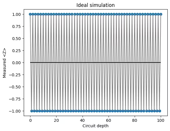
2.6 סימולציה אידיאלית

ideal_sampler = Sampler()
job_ideal = ideal_sampler.run(circuits)
result_ideal = job_ideal.result()
plt.title("Ideal simulation")
ds = list(range(MAX_DEPTH + 1))
plt.plot(
    ds,
    [result_ideal[d].data.meas.expectation_values(["Z"]) for d in ds],
    color="gray",
    linestyle="-",
)
plt.scatter(
    ds, [result_ideal[d].data.meas.expectation_values(["Z"]) for d in ds], marker="o"
)
plt.hlines(0, xmin=0, xmax=MAX_DEPTH, colors="black")
plt.xlabel("Circuit depth")
plt.ylabel("Measured <Z>")
plt.show()

2.7 תרגיל

על ידי שינוי הקוד להלן,

• נסה 25 פעמים יותר shots (= 10_000 shots) וודא שמתקבל גרף חלק יותר
• שנה פרמטרי רעש (OVER_ROTATION_ANGLE, AMPLITUDE_DAMPING_PARAM, PREP0_MEAS1, או PREP1_MEAS0) וראה כיצד הגרף משתנה

OVER_ROTATION_ANGLE = 0.05
coherent_error = coherent_unitary_error(RXGate(OVER_ROTATION_ANGLE).to_matrix())
AMPLITUDE_DAMPING_PARAM = 0.02  # in [0, 1] (0: no error)
incoherent_error = amplitude_damping_error(AMPLITUDE_DAMPING_PARAM)
PREP0_MEAS1 = 0.1  # P(1|0): Probability of preparing 0 and measuring 1
PREP1_MEAS0 = 0.05  # P(0|1): Probability of preparing 1 and measuring 0
readout_error = ReadoutError(
    [[1 - PREP0_MEAS1, PREP0_MEAS1], [PREP1_MEAS0, 1 - PREP1_MEAS0]]
)
noise_model = NoiseModel()
noise_model.add_quantum_error(coherent_error.compose(incoherent_error), "x", (0,))
noise_model.add_readout_error(readout_error, (0,))
options = {
    "backend_options": {"noise_model": noise_model},
}
noisy_sampler = Sampler(options=options)
job = noisy_sampler.run(circuits, shots=400)
result = job.result()
plt.title("Noisy simulation")
ds = list(range(MAX_DEPTH + 1))
plt.plot(
    ds,
    [result[d].data.meas.expectation_values(["Z"]) for d in ds],
    marker="o",
    linestyle="-",
)
plt.hlines(0, xmin=0, xmax=MAX_DEPTH, colors="black")
plt.ylim(-1, 1)
plt.xlabel("Depth")
plt.ylabel("Measured <Z>")
plt.show()

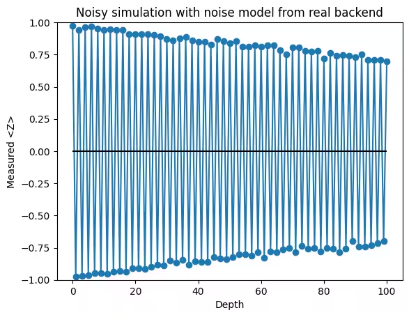
2.8 סימולציה רועשת ריאליסטית יותר

from qiskit_aer import AerSimulator
from qiskit_ibm_runtime import SamplerV2 as Sampler, QiskitRuntimeService

service = QiskitRuntimeService()
real_backend = service.least_busy(
    operational=True, simulator=False, min_num_qubits=127
)  # Eagle

<IBMBackend('ibm_strasbourg')>

aer = AerSimulator.from_backend(real_backend)
noisy_sampler = Sampler(mode=aer)
job = noisy_sampler.run(circuits)
result = job.result()
plt.title("Noisy simulation with noise model from real backend")
ds = list(range(MAX_DEPTH + 1))
plt.plot(
    ds,
    [result[d].data.meas.expectation_values(["Z"]) for d in ds],
    marker="o",
    linestyle="-",
)
plt.hlines(0, xmin=0, xmax=MAX_DEPTH, colors="black")
plt.ylim(-1, 1)
plt.xlabel("Depth")
plt.ylabel("Measured <Z>")
plt.show()

3. חישוב קוונטי אמיתי עם הפחתת שגיאות

בחלק הזה, נדגים איך לקבל תוצאות עם הפחתת שגיאות (ערכי ציפייה) באמצעות Qiskit Estimator. אנחנו מסתכלים על Circuit-ים של Trotterized בגודל 6 Qubit-ים לסימולציית האבולוציה הזמנית של מודל Ising חד-ממדי, ורואים איך השגיאה מתרחבת ביחס למספר צעדי הזמן.

backend = service.least_busy(
    operational=True, simulator=False, min_num_qubits=127
)  # Eagle
backend

<IBMBackend('ibm_strasbourg')>

NUM_QUBITS = 6
NUM_TIME_STEPS = list(range(8))
RX_ANGLE = 0.1
RZZ_ANGLE = 0.1

3.1 בניית Circuit-ים

# Build circuits with different number of time steps
circuits = []
for n_steps in NUM_TIME_STEPS:
    circ = QuantumCircuit(NUM_QUBITS)
    for i in range(n_steps):
        # rx layer
        for q in range(NUM_QUBITS):
            circ.rx(RX_ANGLE, q)
        # 1st rzz layer
        for q in range(1, NUM_QUBITS - 1, 2):
            circ.rzz(RZZ_ANGLE, q, q + 1)
        # 2nd rzz layer
        for q in range(0, NUM_QUBITS - 1, 2):
            circ.rzz(RZZ_ANGLE, q, q + 1)
    circ.barrier()  # need not to optimize the circuit
    # Uncompute stage
    for i in range(n_steps):
        for q in range(0, NUM_QUBITS - 1, 2):
            circ.rzz(-RZZ_ANGLE, q, q + 1)
        for q in range(1, NUM_QUBITS - 1, 2):
            circ.rzz(-RZZ_ANGLE, q, q + 1)
        for q in range(NUM_QUBITS):
            circ.rx(-RX_ANGLE, q)
    circuits.append(circ)

כדי לדעת מראש מה הפלט האידיאלי, אנחנו משתמשים ב-Circuit-ים מסוג compute-uncompute שמורכבים משלב ראשון שבו מוחל ה-Circuit המקורי $U$, ושלב שני שבו הוא הופך $U^\dagger$. שימו לב שהתוצאה האידיאלית של Circuit-ים כאלה תהיה באופן טריוויאלי מצב הכניסה $|000000\rangle$, שיש לו ערכי ציפייה טריוויאליים לכל אבזרי Pauli, למשל $\langle IIIIIZ \rangle = 1$.

# Print the circuit with 2 time steps
circuits[2].draw(output="mpl")

שימו לב: כפי שמוצג למעלה, ל-Circuit עם $k$ צעדי זמן יהיו $4k$ שכבות של Gate-ים דו-Qubit.

obs = SparsePauliOp.from_sparse_list([("Z", [0], 1.0)], num_qubits=NUM_QUBITS)
obs

SparsePauliOp(['IIIIIZ'],
              coeffs=[1.+0.j])

3.2 Transpile של ה-Circuit-ים

אנחנו מבצעים Transpile על ה-Circuit-ים עבור ה-Backend עם אופטימיזציה (optimization_level=1).

from qiskit.transpiler.preset_passmanagers import generate_preset_pass_manager

pm = generate_preset_pass_manager(optimization_level=1, backend=backend)
isa_circuits = pm.run(circuits)
display(isa_circuits[2].draw("mpl", idle_wires=False, fold=-1))

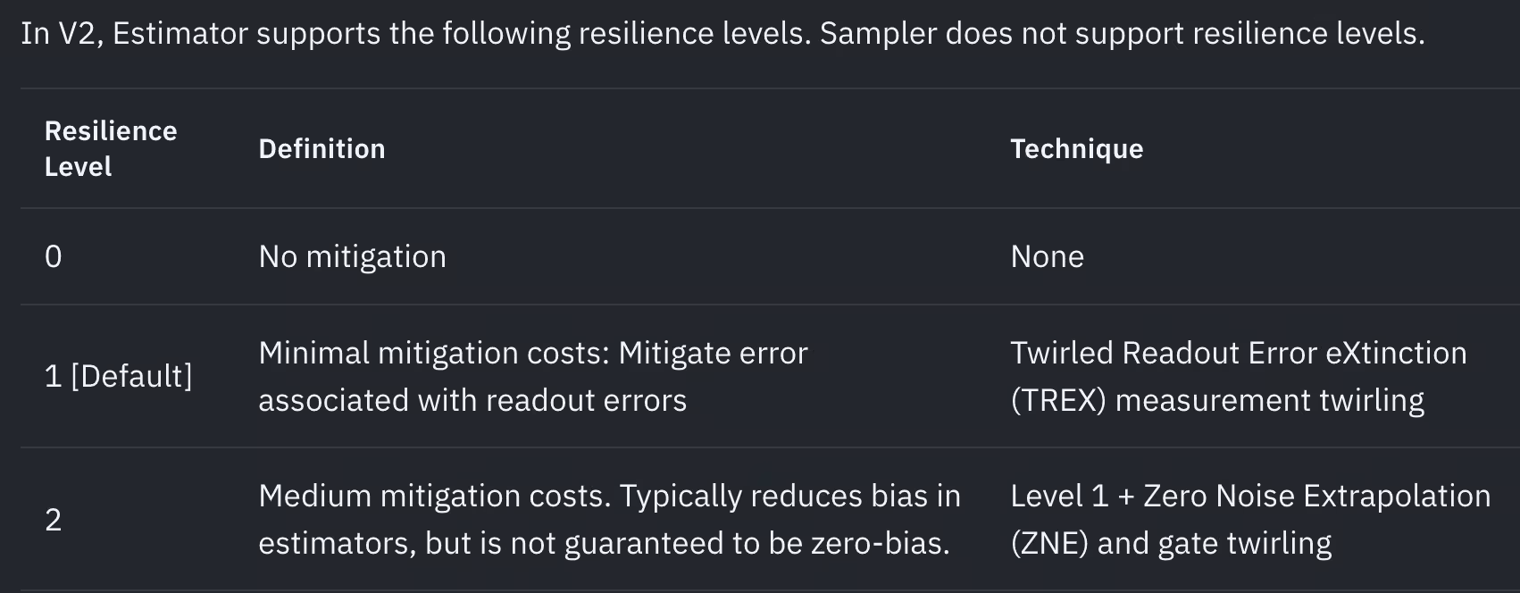
3.3 הרצה באמצעות Estimator (עם רמות resilience שונות)

הגדרת רמת ה-resilience (estimator.options.resilience_level) היא הדרך הקלה ביותר להחיל הפחתת שגיאות כשמשתמשים ב-Qiskit Estimator. ה-Estimator תומך ברמות ה-resilience הבאות (נכון ל-28/06/2024). ראו פרטים נוספים במדריך הגדרת הפחתת שגיאות.

from qiskit_ibm_runtime import Batch
from qiskit_ibm_runtime import EstimatorV2 as Estimator

jobs = []
job_ids = []
with Batch(backend=backend):
    for resilience_level in [0, 1, 2]:
        estimator = Estimator()
        estimator.options.resilience_level = resilience_level
        job = estimator.run(
            [(circ, obs.apply_layout(circ.layout)) for circ in isa_circuits]
        )
        job_ids.append(job.job_id())
        print(f"Job ID (rl={resilience_level}): {job.job_id()}")
        jobs.append(job)

Job ID (rl=0): d146vcnmya70008emprg
Job ID (rl=1): d146vdnqf56g0081sva0
Job ID (rl=2): d146ven5z6q00087c61g

# check job status
for job in jobs:
    print(job.status())

DONE
DONE
DONE

# REPLACE WITH YOUR OWN JOB IDS
jobs = [service.job(job_id) for job_id in job_ids]

# Get results
results = [job.result() for job in jobs]

3.4 הצגת התוצאות בגרף

plt.title("Error mitigation with different resilience levels")
labels = ["0 (No mitigation)", "1 (TREX)", "2 (ZNE + Gate twirling)"]
steps = NUM_TIME_STEPS
for result, label in zip(results, labels):
    plt.errorbar(
        x=steps,
        y=[result[s].data.evs for s in steps],
        yerr=[result[s].data.stds for s in steps],
        marker="o",
        linestyle="-",
        capsize=4,
        label=label,
    )
plt.hlines(
    1.0, min(steps), max(steps), linestyle="dashed", label="Ideal", colors="black"
)
plt.xlabel("Time steps")
plt.ylabel("Mitigated <IIIIIZ>")
plt.legend()
plt.show()

4. (אופציונלי) התאמה אישית של אפשרויות הפחתת שגיאות

אפשר להתאים אישית את החלת טכניקות הפחתת השגיאות דרך אפשרויות כפי שמוצג להלן.

# TREX
estimator.options.twirling.enable_measure = True
estimator.options.twirling.num_randomizations = "auto"
estimator.options.twirling.shots_per_randomization = "auto"

# Gate twirling
estimator.options.twirling.enable_gates = True
# ZNE
estimator.options.resilience.zne_mitigation = True
estimator.options.resilience.zne.noise_factors = [1, 3, 5]
estimator.options.resilience.zne.extrapolator = ("exponential", "linear")

# Dynamical decoupling
estimator.options.dynamical_decoupling.enable = True  # Default: False
estimator.options.dynamical_decoupling.sequence_type = "XX"

# Other options
estimator.options.default_shots = 10_000

ראו את המדריכים ואת ה-API reference הבאים לפרטים על אפשרויות הפחתת השגיאות.

• הגדרת הפחתת שגיאות
• מבוא לאפשרויות
• EstimatorOptions
• SamplerOptions