סימולציה קוונטית

הערה

Yukio Kawashima (May 30, 2024)

הורד את ה-PDF של ההרצאה המקורית. שים לב שחלק מקטעי הקוד עשויים להיות מיושנים מכיוון שאלו תמונות סטטיות.

זמן QPU משוער להרצת הניסוי הוא 7 שניות.

(מחברת זו לקוחה ברובה ממחברת הדרכה שהוצאה משימוש עבור Qiskit Algorithms.)

1. מבוא

כטכניקת אבולוציה בזמן אמת, טרוטריזציה מורכבת מהפעלה עוקבת של Gate קוונטי אחד או יותר, שנבחרו לקירוב האבולוציה בזמן של מערכת עבור פרוסת זמן. בעקבות משוואת שרדינגר, האבולוציה בזמן של מערכת שנמצאת בתחילה במצב $\vert\psi(0)\rangle$ לובשת את הצורה:

$$\vert \psi(t) \rangle = e^{-i H t} \vert \psi(0) \rangle \text{,}$$

כאשר $H$ הוא ההמילטוניאן הבלתי תלוי בזמן המנהל את המערכת. אנו מתייחסים להמילטוניאן שניתן לכתוב כסכום משוקלל של איברי פאולי $H=\sum_j a_j P_j$, כאשר $P_j$ מייצג מכפלה טנזורית של איברי פאולי הפועלים על $n$ Qubits. בפרט, ייתכן שאיברי פאולי אלו מתחלפים זה עם זה, וייתכן שלא. בהינתן מצב בזמן $t=0$, כיצד מקבלים את מצב המערכת בזמן מאוחר יותר $|\psi(t)\rangle$ באמצעות מחשב קוונטי? את האקספוננט של אופרטור ניתן להבין בצורה הקלה ביותר דרך טור טיילור שלו:

$$e^{-i H t} = 1-iHt-\frac{1}{2}H^2t^2+...$$

אקספוננטים בסיסיים מאוד, כמו $e^{iZ}$, ניתנים לממוש בקלות במחשבים קוונטיים באמצעות קבוצה קומפקטית של Gates קוונטיים. לרוב ההמילטוניאנים המעניינים לא יהיה רק איבר בודד, אלא הרבה איברים. שימו לב למה שקורה כאשר $H = H_1+H_2$:

$$e^{-i H t} = 1-i(H_1+H_2)t-\frac{1}{2}(H_1+H_2)^2t^2+...$$

כאשר $H_1$ ו-$H_2$ מתחלפים, יש לנו את המקרה המוכר (שתקף גם למספרים, ולמשתנים $a$ ו-$b$ להלן):

$$e^{-i (a+b) t} = e^{-i a t}e^{-i b t}$$

אבל כאשר אופרטורים אינם מתחלפים, לא ניתן לסדר מחדש את האיברים בטור טיילור כדי לפשט בדרך זו. לפיכך, ביטוי המילטוניאנים מסובכים בעזרת Gates קוונטיים הוא אתגר.

פתרון אחד הוא לשקול זמן קצר מאוד $t$, כך שהאיבר מסדר ראשון בפיתוח טיילור שולט. תחת הנחה זו:

$$e^{-i (H_1+H_2) t} \approx 1-i(H_1+H_2)t \approx (1-i H_1 t)(1-i H_2 t) \approx e^{-i H_1 t}e^{-i H_2 t}$$

כמובן, ייתכן שנצטרך לאפשר למערכת להתפתח על פני זמן ארוך יותר. זה מושג על ידי שימוש בצעדים קטנים רבים בזמן. תהליך זה נקרא טרוטריזציה:

$$\vert \psi(t) \rangle \approx \left(\prod_j e^{-i a_j P_j t/r} \right)^r \vert\psi(0) \rangle \text{,}$$

כאן $t/r$ הוא פרוסת הזמן (צעד האבולוציה) שאנו בוחרים. כתוצאה מכך, נוצר Gate שמופעל $r$ פעמים. צעד זמן קטן יותר מוביל לקירוב מדויק יותר. עם זאת, הדבר גם מוביל ל-Circuits עמוקים יותר, אשר בפועל גורמים לצבירת שגיאות גדולה יותר (דאגה לא מבוטלת על מכשירים קוונטיים מהדור הנוכחי).

היום נלמד את האבולוציה בזמן של מודל איזינג על סריגים לינאריים עם $N=2$ ו-$N=6$ אתרים. סריגים אלו מורכבים ממערך של ספינים $\sigma_i$ המקיימים אינטראקציה רק עם שכניהם הקרובים ביותר. לספינים אלו יכולות להיות שתי אוריינטציות: $\uparrow$ ו-$\downarrow$, המתאימות למגנטיזציה של $+1$ ו-$-1$ בהתאמה.

$$H = - J \sum_{i=0}^{N-2} Z_i Z_{i+1} - h \sum_{i=0}^{N-1} X_i \text{,}$$

כאשר $J$ מתאר את אנרגיית האינטראקציה, ו-$h$ את עצמת השדה החיצוני (בכיוון ה-x לעיל, אך נשנה זאת). בואו נכתוב ביטוי זה באמצעות מטריצות פאולי, תוך התחשבות בכך שלשדה החיצוני יש זווית $\alpha$ ביחס לכיוון הרוחבי,

$$H = -J \sum_{i=0}^{N-2} Z_i Z_{i+1} -h \sum_{i=0}^{N-1} (\sin\alpha Z_i + \cos\alpha X_i) \text{.}$$

המילטוניאן זה שימושי בכך שהוא מאפשר לנו לחקור בקלות את השפעות השדה החיצוני. בבסיס החישובי, המערכת תקודד באופן הבא:

מצב קוונטי	ייצוג ספינים
$\lvert 0 0 0 0 \rangle$	$\uparrow\uparrow\uparrow\uparrow$
$\lvert 1 0 0 0 \rangle$	$\downarrow\uparrow\uparrow\uparrow$
$\ldots$	$\ldots$
$\lvert 1 1 1 1 \rangle$	$\downarrow\downarrow\downarrow\downarrow$

נתחיל לחקור את האבולוציה בזמן של מערכת קוונטית כזו. ליתר דיוק, נדמיין את האבולוציה בזמן של תכונות מסוימות של המערכת כמו מגנטיזציה.

1.1 דרישות

לפני תחילת הדרכה זו, וודאו שהכלים הבאים מותקנים:

• Qiskit SDK v1.2 ומעלה ( pip install qiskit )
• Qiskit Runtime v0.30 ומעלה ( pip install qiskit-ibm-runtime )
• Numpy v1.24.1 ומעלה < 2 ( pip install numpy )

1.2 ייבוא הספריות

שימו לב שחלק מהספריות שעשויות להיות שימושיות (MatrixExponential, QDrift) נכללות למרות שאינן בשימוש במחברת הנוכחית. אתם יכולים לנסות אותן אם יש לכם זמן!

# Added by doQumentation — required packages for this notebook
!pip install -q matplotlib numpy qiskit qiskit-ibm-runtime

# Check the version of Qiskit
import qiskit

qiskit.__version__

'2.0.2'

# Import the qiskit library
import numpy as np
import matplotlib.pylab as plt
import warnings

from qiskit import QuantumCircuit
from qiskit.circuit.library import PauliEvolutionGate
from qiskit.primitives import StatevectorEstimator
from qiskit.quantum_info import Statevector, SparsePauliOp
from qiskit.synthesis import (
    SuzukiTrotter,
    LieTrotter,
)
from qiskit.transpiler.preset_passmanagers import generate_preset_pass_manager

from qiskit_ibm_runtime import QiskitRuntimeService, SamplerV2

warnings.filterwarnings("ignore")

2. מיפוי הבעיה

2.1 הגדרת ההמילטוניאן של מודל איזינג בשדה רוחבי

אנו מתייחסים כאן למודל איזינג חד-ממדי בשדה רוחבי.

ראשית, ניצור פונקציה שמקבלת את פרמטרי המערכת $N$, $J$, $h$ ו-$\alpha$, ומחזירה את ההמילטוניאן שלנו כ-SparsePauliOp. SparsePauliOp הוא ייצוג דליל של אופרטור במונחים של איברי Pauli משוקללים.

def get_hamiltonian(nqubits, J, h, alpha):
    # List of Hamiltonian terms as 3-tuples containing
    # (1) the Pauli string,
    # (2) the qubit indices corresponding to the Pauli string,
    # (3) the coefficient.
    ZZ_tuples = [("ZZ", [i, i + 1], -J) for i in range(0, nqubits - 1)]
    Z_tuples = [("Z", [i], -h * np.sin(alpha)) for i in range(0, nqubits)]
    X_tuples = [("X", [i], -h * np.cos(alpha)) for i in range(0, nqubits)]

    # We create the Hamiltonian as a SparsePauliOp, via the method
    # `from_sparse_list`, and multiply by the interaction term.
    hamiltonian = SparsePauliOp.from_sparse_list(
        [*ZZ_tuples, *Z_tuples, *X_tuples], num_qubits=nqubits
    )
    return hamiltonian.simplify()

הגדרת ההמילטוניאן

המערכת שאנו מתייחסים אליה כעת היא בגודל $N=6$, $J=0.2$, $h=1.2$ ו-$\alpha=\frac{\pi}{8.0}$ כדוגמה.

n_qubits = 6

hamiltonian = get_hamiltonian(nqubits=n_qubits, J=0.2, h=1.2, alpha=np.pi / 8.0)
hamiltonian

SparsePauliOp(['IIIIZZ', 'IIIZZI', 'IIZZII', 'IZZIII', 'ZZIIII', 'IIIIIZ', 'IIIIZI', 'IIIZII', 'IIZIII', 'IZIIII', 'ZIIIII', 'IIIIIX', 'IIIIXI', 'IIIXII', 'IIXIII', 'IXIIII', 'XIIIII'],
              coeffs=[-0.2       +0.j, -0.2       +0.j, -0.2       +0.j, -0.2       +0.j,
 -0.2       +0.j, -0.45922012+0.j, -0.45922012+0.j, -0.45922012+0.j,
 -0.45922012+0.j, -0.45922012+0.j, -0.45922012+0.j, -1.10865544+0.j,
 -1.10865544+0.j, -1.10865544+0.j, -1.10865544+0.j, -1.10865544+0.j,
 -1.10865544+0.j])

2.2 הגדרת פרמטרי סימולציית האבולוציה בזמן

כאן נשקול שלוש טכניקות טרוטריזציה שונות:

• Lie–Trotter (סדר ראשון)
• Suzuki–Trotter מסדר שני
• Suzuki–Trotter מסדר רביעי

שתיים האחרונות ישמשו בתרגיל ובנספח.

num_timesteps = 60
evolution_time = 30.0
dt = evolution_time / num_timesteps
product_formula_lt = LieTrotter()
product_formula_st2 = SuzukiTrotter(order=2)
product_formula_st4 = SuzukiTrotter(order=4)

2.3 הכנת ה-Circuit הקוונטי 1 (מצב התחלתי)

יצירת מצב התחלתי. כאן נתחיל עם קונפיגורציית הספינים $\uparrow\uparrow\downarrow\downarrow\uparrow\uparrow$ .

initial_circuit = QuantumCircuit(n_qubits)
initial_circuit.prepare_state("001100")
# Change reps and see the difference when you decompose the circuit
initial_circuit.decompose(reps=1).draw("mpl")

2.4 הכנת ה-Circuit הקוונטי 2 (Circuit יחיד לאבולוציה בזמן)

אנו בונים כאן Circuit עבור צעד זמן בודד תוך שימוש ב-Lie–Trotter.

נוסחת המכפלה של Lie (סדר ראשון) מממושת במחלקה LieTrotter. נוסחה מסדר ראשון מורכבת מהקירוב שצוין במבוא, שבו האקספוננט המטריצי של סכום מקורב על ידי מכפלה של אקספוננטים מטריציים:

$$e^{H_1+H_2} \approx e^{H_1} e^{H_2}$$

כפי שצוין קודם, Circuits עמוקים מאוד מובילים לצבירת שגיאות, וגורמים לבעיות עבור מחשבים קוונטיים מודרניים. מכיוון ש-Gates דו-Qubit מכילים שיעורי שגיאות גבוהים יותר מ-Gates חד-Qubit, כמות מעניינת במיוחד היא עומק ה-Circuit הדו-Qubit. מה שחשוב באמת הוא עומק ה-Circuit הדו-Qubit לאחר Transpilation (מכיוון שזהו ה-Circuit שהמחשב הקוונטי מבצע בפועל). אבל בואו נרגיל את עצמנו לספור את הפעולות עבור ה-Circuit הזה, גם כעת בשימוש בסימולטור.

single_step_evolution_gates_lt = PauliEvolutionGate(
    hamiltonian, dt, synthesis=product_formula_lt
)
single_step_evolution_lt = QuantumCircuit(n_qubits)
single_step_evolution_lt.append(
    single_step_evolution_gates_lt, single_step_evolution_lt.qubits
)

print(
    f"""
Trotter step with Lie-Trotter
-----------------------------
Depth: {single_step_evolution_lt.decompose(reps=3).depth()}
Gate count: {len(single_step_evolution_lt.decompose(reps=3))}
Nonlocal gate count: {single_step_evolution_lt.decompose(reps=3).num_nonlocal_gates()}
Gate breakdown: {", ".join([f"{k.upper()}: {v}" for k, v in single_step_evolution_lt.decompose(reps=3).count_ops().items()])}
"""
)
single_step_evolution_lt.decompose(reps=3).draw("mpl", fold=-1)

Trotter step with Lie-Trotter
-----------------------------
Depth: 17
Gate count: 27
Nonlocal gate count: 10
Gate breakdown: U3: 12, CX: 10, U1: 5

2.5 הגדרת האופרטורים למדידה

בואו נגדיר אופרטור מגנטיזציה $\sum_i \langle Z_i \rangle / N$, ו-אופרטור מתאם ספינים ממוצע $\sum_i \langle Z_i Z_{i+1} \rangle/ (N - 1)$.

magnetization = (
    SparsePauliOp.from_sparse_list(
        [("Z", [i], 1.0) for i in range(0, n_qubits)], num_qubits=n_qubits
    )
    / n_qubits
)
correlation = SparsePauliOp.from_sparse_list(
    [("ZZ", [i, i + 1], 1.0) for i in range(0, n_qubits - 1)], num_qubits=n_qubits
) / (n_qubits - 1)
print("magnetization : ", magnetization)
print("correlation : ", correlation)

magnetization :  SparsePauliOp(['IIIIIZ', 'IIIIZI', 'IIIZII', 'IIZIII', 'IZIIII', 'ZIIIII'],
              coeffs=[0.16666667+0.j, 0.16666667+0.j, 0.16666667+0.j, 0.16666667+0.j,
 0.16666667+0.j, 0.16666667+0.j])
correlation :  SparsePauliOp(['IIIIZZ', 'IIIZZI', 'IIZZII', 'IZZIII', 'ZZIIII'],
              coeffs=[0.2+0.j, 0.2+0.j, 0.2+0.j, 0.2+0.j, 0.2+0.j])

2.6 ביצוע סימולציית האבולוציה בזמן

נעקוב אחר האנרגיה (ערך הציפייה של ההמילטוניאן), המגנטיזציה (ערך הציפייה של אופרטור המגנטיזציה), ומתאם הספינים הממוצע (ערך הציפייה של אופרטור מתאם הספינים הממוצע). ה-StatevectorEstimator (EstimatorV2) של Qiskit מעריך ערכי ציפייה של אובייקטים, $\langle\psi\vert\hat{O}\vert\psi\rangle$.

# Initiate the circuit
evolved_state = QuantumCircuit(initial_circuit.num_qubits)
# Start from the initial spin configuration
evolved_state.append(initial_circuit, evolved_state.qubits)
# Initiate Estimator (V2)
estimator = StatevectorEstimator()
# Set number of shots
shots = 10000
# Translate the precision required from the number of shots
precision = np.sqrt(1 / shots)
energy_list = []
mag_list = []
corr_list = []
# Estimate expectation values for t=0.0
job = estimator.run(
    [(evolved_state, [hamiltonian, magnetization, correlation])], precision=precision
)
# Get estimated expectation values
evs = job.result()[0].data.evs
energy_list.append(evs[0])
mag_list.append(evs[1])
corr_list.append(evs[2])
# Start time evolution
for n in range(num_timesteps):
    # Expand the circuit to describe delta-t
    evolved_state.append(single_step_evolution_gates_lt, evolved_state.qubits)
    # Estimate expectation values at delta-t
    job = estimator.run(
        [(evolved_state, [hamiltonian, magnetization, correlation])],
        precision=precision,
    )
    # Retrieve results (expectation values)
    evs = job.result()[0].data.evs
    energy_list.append(evs[0])
    mag_list.append(evs[1])
    corr_list.append(evs[2])
# Transform the list of expectation values (at each time step) to arrays
energy_array = np.array(energy_list)
mag_array = np.array(mag_list)
corr_array = np.array(corr_list)

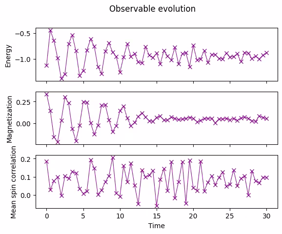
2.7 שרטוט האבולוציה בזמן של האובייקטים

נשרטט את ערכי הציפייה שמדדנו כנגד הזמן.

fig, axes = plt.subplots(3, sharex=True)
times = np.linspace(0, evolution_time, num_timesteps + 1)  # includes initial state
axes[0].plot(
    times,
    energy_array,
    label="First order",
    marker="x",
    c="darkmagenta",
    ls="-",
    lw=0.8,
)
axes[1].plot(
    times, mag_array, label="First order", marker="x", c="darkmagenta", ls="-", lw=0.8
)
axes[2].plot(
    times, corr_array, label="First order", marker="x", c="darkmagenta", ls="-", lw=0.8
)
axes[0].set_ylabel("Energy")
axes[1].set_ylabel("Magnetization")
axes[2].set_ylabel("Mean spin correlation")
axes[2].set_xlabel("Time")
fig.suptitle("Observable evolution")

Text(0.5, 0.98, 'Observable evolution')

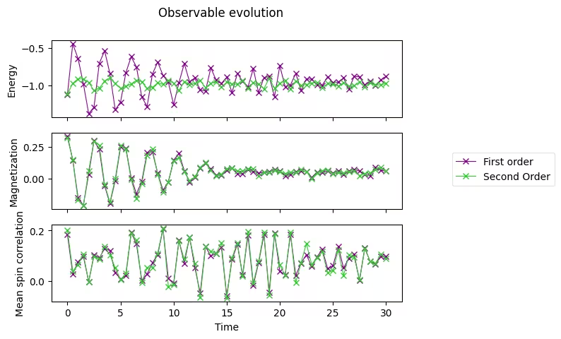
3. תרגיל 1. ביצוע סימולציה באמצעות Suzuki–Trotter מסדר שני

עכשיו בואו ננסה לבצע סימולציה עם Suzuki–Trotter מסדר שני בהמשך לדוגמה של Lie–Trotter שראינו למעלה.

ניתן להשתמש ב-Suzuki-Trotter מסדר שני ב-Qiskit באמצעות מחלקת SuzukiTrotter. בשימוש בנוסחה זו, פירוק מסדר שני הוא:

$$e^{H_1+H_2} \approx e^{H_1/2}e^{H_2}e^{H_1/2}$$

3.1 בניית Circuit לצעד זמן יחיד

השתמש ב-product_formula_st2 (SuzukiTrotter(order=2)) ובנה Circuit לצעד זמן יחיד עם Suzuki–Trotter מסדר שני. כמו כן, ספור את מספר ה-Gate-ים ואת עומק ה-Circuit והשווה עם Lie–Trotter.

# Modify the line below (Use PauliEvolutionGate)
single_step_evolution_gates_st2 = PauliEvolutionGate(
    hamiltonian, dt, synthesis=product_formula_st2
)
single_step_evolution_st2 = QuantumCircuit(n_qubits)
single_step_evolution_st2.append(
    single_step_evolution_gates_st2, single_step_evolution_st2.qubits
)
# Let us print some stats
print(
    f"""
Trotter step with second-order Suzuki-Trotter
-----------------------------
Depth: {single_step_evolution_st2.decompose(reps=3).depth()}
Gate count: {len(single_step_evolution_st2.decompose(reps=3))}
Nonlocal gate count: {single_step_evolution_st2.decompose(reps=3).num_nonlocal_gates()}
Gate breakdown: {", ".join([f"{k.upper()}: {v}" for k, v in single_step_evolution_st2.decompose(reps=3).count_ops().items()])}
"""
)
single_step_evolution_st2.decompose(reps=2).draw("mpl", fold=-1)

Trotter step with second-order Suzuki-Trotter
-----------------------------
Depth: 34
Gate count: 53
Nonlocal gate count: 20
Gate breakdown: U3: 23, CX: 20, U1: 10

3.2 ביצוע סימולציית התפתחות בזמן

בצע התפתחות בזמן עם Suzuki–Trotter מסדר שני.

# Initiate the circuit
evolved_state = QuantumCircuit(initial_circuit.num_qubits)
# Start from the initial spin configuration
evolved_state.append(initial_circuit, evolved_state.qubits)
# Initiate Estimator (V2)
estimator = StatevectorEstimator()
# Set number of shots
shots = 10000
# Translate the precision required from the number of shots
precision = np.sqrt(1 / shots)
energy_list_st2 = []
mag_list_st2 = []
corr_list_st2 = []
# Estimate expectation values for t=0.0
job = estimator.run(
    [(evolved_state, [hamiltonian, magnetization, correlation])], precision=precision
)
# Get estimated expectation values
evs = job.result()[0].data.evs
energy_list_st2.append(evs[0])
mag_list_st2.append(evs[1])
corr_list_st2.append(evs[2])
# Start time evolution
for n in range(num_timesteps):
    # Expand the circuit to describe delta-t
    evolved_state.append(single_step_evolution_gates_st2, evolved_state.qubits)
    # Estimate expectation values at delta-t
    job = estimator.run(
        [(evolved_state, [hamiltonian, magnetization, correlation])],
        precision=precision,
    )
    # Retrieve results (expectation values)
    evs = job.result()[0].data.evs
    energy_list_st2.append(evs[0])
    mag_list_st2.append(evs[1])
    corr_list_st2.append(evs[2])
# Transform the list of expectation values (at each time step) to arrays
energy_array_st2 = np.array(energy_list_st2)
mag_array_st2 = np.array(mag_list_st2)
corr_array_st2 = np.array(corr_list_st2)

3.3 הצגת תוצאות Suzuki–Trotter מסדר שני

axes[0].plot(
    times,
    energy_array_st2,
    label="Second Order",
    marker="x",
    c="limegreen",
    ls="-",
    lw=0.8,
)
axes[1].plot(
    times,
    mag_array_st2,
    label="Second Order",
    marker="x",
    c="limegreen",
    ls="-",
    lw=0.8,
)
axes[2].plot(
    times,
    corr_array_st2,
    label="Second Order",
    marker="x",
    c="limegreen",
    ls="-",
    lw=0.8,
)

# Replace the legend
# legend.remove()
legend = fig.legend(
    *axes[0].get_legend_handles_labels(),
    bbox_to_anchor=(1.0, 0.5),
    loc="center left",
    framealpha=0.5,
)
fig

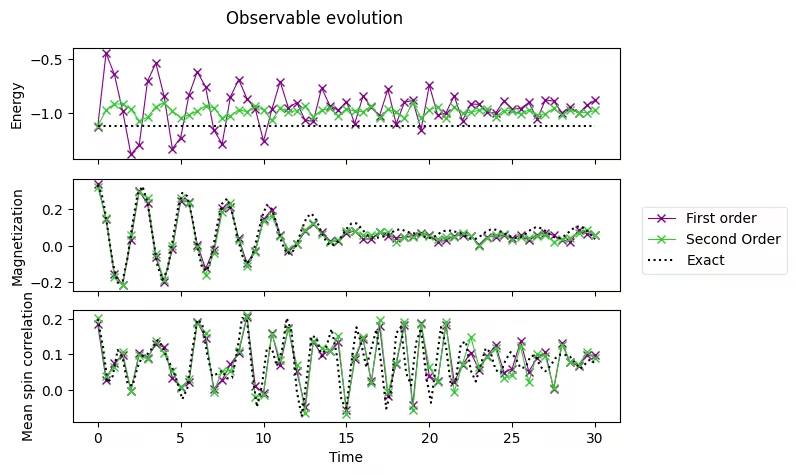
3.4 השוואה עם תוצאות מדויקות

הנתונים שלהלן הם התוצאות המדויקות שחושבו מראש על ידי המחשב הקלאסי.

exact_times = np.array(
    [
        0.0,
        0.3,
        0.6,
        0.8999999999999999,
        1.2,
        1.5,
        1.7999999999999998,
        2.1,
        2.4,
        2.6999999999999997,
        3.0,
        3.3,
        3.5999999999999996,
        3.9,
        4.2,
        4.5,
        4.8,
        5.1,
        5.3999999999999995,
        5.7,
        6.0,
        6.3,
        6.6,
        6.8999999999999995,
        7.199999999999999,
        7.5,
        7.8,
        8.1,
        8.4,
        8.7,
        9.0,
        9.299999999999999,
        9.6,
        9.9,
        10.2,
        10.5,
        10.799999999999999,
        11.1,
        11.4,
        11.7,
        12.0,
        12.299999999999999,
        12.6,
        12.9,
        13.2,
        13.5,
        13.799999999999999,
        14.1,
        14.399999999999999,
        14.7,
        15.0,
        15.299999999999999,
        15.6,
        15.899999999999999,
        16.2,
        16.5,
        16.8,
        17.099999999999998,
        17.4,
        17.7,
        18.0,
        18.3,
        18.599999999999998,
        18.9,
        19.2,
        19.5,
        19.8,
        20.099999999999998,
        20.4,
        20.7,
        21.0,
        21.3,
        21.599999999999998,
        21.9,
        22.2,
        22.5,
        22.8,
        23.099999999999998,
        23.4,
        23.7,
        24.0,
        24.3,
        24.599999999999998,
        24.9,
        25.2,
        25.5,
        25.8,
        26.099999999999998,
        26.4,
        26.7,
        27.0,
        27.3,
        27.599999999999998,
        27.9,
        28.2,
        28.5,
        28.799999999999997,
        29.099999999999998,
        29.4,
        29.7,
        30.0,
    ]
)
exact_energy = np.array(
    [
        -1.1184402376762155,
        -1.1184402376762157,
        -1.1184402376762157,
        -1.1184402376762148,
        -1.1184402376762153,
        -1.1184402376762155,
        -1.1184402376762148,
        -1.118440237676216,
        -1.118440237676216,
        -1.1184402376762166,
        -1.1184402376762148,
        -1.118440237676216,
        -1.1184402376762153,
        -1.1184402376762148,
        -1.118440237676217,
        -1.118440237676215,
        -1.1184402376762161,
        -1.1184402376762157,
        -1.118440237676217,
        -1.1184402376762161,
        -1.1184402376762137,
        -1.1184402376762161,
        -1.1184402376762161,
        -1.118440237676218,
        -1.1184402376762155,
        -1.1184402376762166,
        -1.1184402376762155,
        -1.1184402376762137,
        -1.1184402376762186,
        -1.1184402376762215,
        -1.1184402376762148,
        -1.118440237676216,
        -1.1184402376762166,
        -1.1184402376762148,
        -1.1184402376762121,
        -1.1184402376762166,
        -1.1184402376762181,
        -1.1184402376762137,
        -1.1184402376762148,
        -1.1184402376762193,
        -1.1184402376762108,
        -1.1184402376762144,
        -1.118440237676217,
        -1.1184402376762197,
        -1.1184402376762153,
        -1.1184402376762161,
        -1.1184402376762184,
        -1.1184402376762126,
        -1.118440237676214,
        -1.118440237676214,
        -1.1184402376762161,
        -1.118440237676212,
        -1.1184402376762164,
        -1.118440237676217,
        -1.1184402376762121,
        -1.1184402376762157,
        -1.1184402376762212,
        -1.1184402376762217,
        -1.1184402376762206,
        -1.118440237676222,
        -1.1184402376762166,
        -1.118440237676212,
        -1.1184402376762137,
        -1.11844023767622,
        -1.1184402376762206,
        -1.118440237676219,
        -1.1184402376762153,
        -1.1184402376762164,
        -1.118440237676209,
        -1.1184402376762144,
        -1.1184402376762161,
        -1.118440237676216,
        -1.1184402376762173,
        -1.118440237676214,
        -1.1184402376762093,
        -1.1184402376762184,
        -1.1184402376762126,
        -1.118440237676213,
        -1.1184402376762195,
        -1.1184402376762095,
        -1.1184402376762075,
        -1.1184402376762197,
        -1.1184402376762141,
        -1.1184402376762146,
        -1.1184402376762184,
        -1.118440237676218,
        -1.1184402376762224,
        -1.118440237676219,
        -1.118440237676218,
        -1.1184402376762206,
        -1.1184402376762168,
        -1.118440237676221,
        -1.118440237676218,
        -1.1184402376762148,
        -1.1184402376762106,
        -1.1184402376762173,
        -1.118440237676216,
        -1.118440237676216,
        -1.1184402376762113,
        -1.1184402376762275,
        -1.1184402376762195,
    ]
)
exact_magnetization = np.array(
    [
        0.3333333333333333,
        0.26316769633415005,
        0.0912947227110664,
        -0.09317712543141576,
        -0.20391854332115245,
        -0.19318196655046493,
        -0.06411527074401464,
        0.12558269854206197,
        0.28252754464640606,
        0.3264196194042506,
        0.2361586169847769,
        0.060894367906122224,
        -0.10842387093076275,
        -0.18636359582538073,
        -0.1338364343947887,
        0.020284606520827753,
        0.19151142743926025,
        0.2905341647678381,
        0.2723014646745304,
        0.15147481733047252,
        -0.008179102877790292,
        -0.1242999208732406,
        -0.1372529247781061,
        -0.04083616185958952,
        0.11066094926716476,
        0.23140661570567636,
        0.2587109403786205,
        0.1868237670027325,
        0.061201779383143744,
        -0.051391248969654205,
        -0.09843899603365061,
        -0.061297056158849166,
        0.04199010081939773,
        0.15861461430963147,
        0.22336830674799552,
        0.20179555623336537,
        0.11407111438609417,
        0.01609419104778282,
        -0.04239611796730001,
        -0.04249123521065924,
        0.008850291714888112,
        0.08780898151558082,
        0.1561486776507056,
        0.17627348772811832,
        0.13870676179652253,
        0.07205869195282538,
        0.018300003064909465,
        0.0001095640839572417,
        0.015157929316037586,
        0.05077755280969454,
        0.09245534457650838,
        0.12206907551110702,
        0.12284950557969157,
        0.09570215398601932,
        0.06294378255078983,
        0.045503313813986014,
        0.043389819499542556,
        0.046725117769796744,
        0.054956411358382404,
        0.0713814528253614,
        0.08743689703248492,
        0.08951216359166674,
        0.07878386475305985,
        0.06955669116405788,
        0.06639892435963689,
        0.05890378761746903,
        0.04541796525844558,
        0.0414221088331947,
        0.05499634106912299,
        0.07409418836014572,
        0.08371859070160165,
        0.08211623987959302,
        0.07615055161378328,
        0.06702584458783024,
        0.051891407742740085,
        0.038049378383635625,
        0.03825614149768043,
        0.054183218463525695,
        0.0753534475741016,
        0.08853147112587295,
        0.08767917178542013,
        0.07709383184439536,
        0.06308595032042386,
        0.0498812359204284,
        0.04299040064096167,
        0.04769159891460652,
        0.06483569572288776,
        0.08698035745435016,
        0.10047391641776235,
        0.09747255683203637,
        0.08098863187287358,
        0.05959496723987331,
        0.04383882265040485,
        0.04232138798062125,
        0.05720514169944535,
        0.08201306299870219,
        0.10274898262000469,
        0.10707552455080133,
        0.09210856128265357,
        0.06379922105742579,
        0.03624325103307953,
    ]
)
exact_correlation = np.array(
    [
        0.2,
        0.1247704225763532,
        0.01943938494098705,
        0.03854917181332821,
        0.11196616231067426,
        0.0906546700356683,
        0.01629373561896267,
        0.011352652889791095,
        0.0636185676540077,
        0.09543834437789013,
        0.10058518161011307,
        0.11829217731417431,
        0.1397812224038133,
        0.12316460402216707,
        0.08541383059335775,
        0.06144846844403662,
        0.020246372880505827,
        -0.02693683090021662,
        0.003919250903281282,
        0.1117419430168554,
        0.19676155181256794,
        0.18594408880783336,
        0.1002673802566004,
        0.03821525827438024,
        0.04485205090247377,
        0.05348102743040269,
        0.03160026140008638,
        0.033437649060464834,
        0.10486939975320728,
        0.20249469538955758,
        0.19735507621013149,
        0.0553097261765083,
        -0.04889114490131667,
        0.011685690974970964,
        0.11705971535823065,
        0.11681165998194759,
        0.06637091239560744,
        0.10936684225958895,
        0.20225454101061405,
        0.16284420833341812,
        -0.0025823294931362067,
        -0.0763416631752919,
        0.02985268630418397,
        0.15234468006771007,
        0.14606385406970995,
        0.0935341856492092,
        0.12325421854361143,
        0.17130422930386324,
        0.10383730044042278,
        -0.031333159406547614,
        -0.05241572078596815,
        0.07722509925347705,
        0.17642188574256007,
        0.12765340239966838,
        0.06309968945093776,
        0.11574687130499339,
        0.16978282647206913,
        0.0736143632571229,
        -0.05356602733119409,
        -0.0009649396796768892,
        0.15921620111869142,
        0.17760366431811037,
        0.04736297330213485,
        0.012122870263181897,
        0.13268065586830521,
        0.1728473023503636,
        0.03999259331072221,
        -0.036997053070222885,
        0.06951528580242439,
        0.1769169993516561,
        0.12290448295710298,
        0.012897784654866427,
        0.02859435620982225,
        0.12895847695150875,
        0.13629536955485938,
        0.05394621059822597,
        0.02298040588184324,
        0.07036499900317271,
        0.11706448623132719,
        0.10435285842074606,
        0.055721236329964965,
        0.04676334743672697,
        0.08417924910022263,
        0.10611161955304965,
        0.089304171047322,
        0.06098589533081194,
        0.06314519797488709,
        0.09431492621892917,
        0.09667836915967139,
        0.0651298357290882,
        0.05176966009147416,
        0.06727229484222669,
        0.08871788283607947,
        0.09907054249093444,
        0.09785167773502176,
        0.09277216140054353,
        0.07520999642062785,
        0.05894392248382922,
        0.07236135251622376,
        0.08608284185200156,
        0.07282922961856123,
    ]
)

axes[0].plot(exact_times, exact_energy, c="k", ls=":", label="Exact")
axes[1].plot(exact_times, exact_magnetization, c="k", ls=":", label="Exact")
axes[2].plot(exact_times, exact_correlation, c="k", ls=":", label="Exact")
# Replace the legend
legend.remove()
# Select the labels of only the first axis
legend = fig.legend(
    *axes[0].get_legend_handles_labels(),
    bbox_to_anchor=(1.0, 0.5),
    loc="center left",
    framealpha=0.5,
)
fig.tight_layout()
fig

4. הרצה על חומרת הקוואנטום

בשלב הבא נריץ את סימולציית האבולוציה בזמן על חומרת הקוואנטום. נעבוד על בעיה קטנה יותר, גודל סריג N=2. נשנה את הפרמטר $\alpha$ ונראה את ההבדל בדינמיקה של פונקציית הגל.

4.1 שלב 1. מיפוי קלטים קלאסיים לבעיה קוואנטית

בחר את ההגדרה הראשונית של הסימולציה:

n_qubits_2 = 2
dt_2 = 1.6
product_formula = LieTrotter(reps=1)

לאחר מכן הגדר את ה-Circuit ההתחלתי:

תצורת הספין ההתחלתית תהיה "למטה-למעלה"

# We prepare an initial state ↓↑ (10).
# Note that Statevector and SparsePauliOp interpret the qubits from right to left
initial_circuit_2 = QuantumCircuit(n_qubits_2)
initial_circuit_2.prepare_state("10")
# Change reps and see the difference when you decompose the circuit
initial_circuit_2.decompose(reps=1).draw("mpl")

כעת חשב את ערך הייחוס באמצעות סימולטור statevector אידיאלי.

bar_width = 0.1
# initial_state = Statevector.from_label("10")
final_time = 1.6
eps = 1e-5

# We create the list of angles in radians, with a small epsilon
# the exactly longitudinal field, which would present no dynamics at all
alphas = np.linspace(-np.pi / 2 + eps, np.pi / 2 - eps, 5)

for i, alpha in enumerate(alphas):
    evolved_state_2 = QuantumCircuit(initial_circuit_2.num_qubits)
    evolved_state_2.append(initial_circuit_2, evolved_state_2.qubits)
    hamiltonian_2 = get_hamiltonian(nqubits=2, J=0.2, h=1.0, alpha=alpha)
    single_step_evolution_gates_2 = PauliEvolutionGate(
        hamiltonian_2, dt_2, synthesis=product_formula
    )
    evolved_state_2.append(single_step_evolution_gates_2, evolved_state_2.qubits)
    evolved_state_2 = Statevector(evolved_state_2)
    # Dictionary of probabilities
    amplitudes_dict = evolved_state_2.probabilities_dict()
    labels = list(amplitudes_dict.keys())
    values = list(amplitudes_dict.values())
    # Convert angle to degrees
    alpha_str = f"$\\alpha={int(np.round(alpha * 180 / np.pi))}^\\circ$"
    plt.bar(np.arange(4) + i * bar_width, values, bar_width, label=alpha_str, alpha=0.7)

plt.xticks(np.arange(4) + 2 * bar_width, labels)
plt.xlabel("Measurement")
plt.ylabel("Probability")
plt.suptitle(
    f"Measurement probabilities at $t={final_time}$, for various field angles $\\alpha$\n"
    f"Initial state: 10, Linear lattice of size $L=2$"
)
plt.legend()

<matplotlib.legend.Legend at 0x11c816590>

הכנו מערכת עם רצף ספינים ראשוני $\downarrow\uparrow$, המתאים ל-$\vert\psi(0)\rangle = \vert10\rangle$. לאחר שאיפשרנו לה להתפתח למשך $t=1.6$ תחת שדה רוחבי ($\alpha=0^\circ$), כמעט בוודאות נמדוד $\uparrow\downarrow$, כלומר, החלפת ספינים. (שים לב שהתוויות מפורשות מימין לשמאל). אם השדה הוא אורכי ($\alpha=\pm90^\circ$), לא תהיה אבולוציה, ולכן נמדוד את המערכת כפי שהוכנה בהתחלה, $\downarrow\uparrow$. בזוויות ביניים, ב-$\alpha=\pm45^\circ$, נוכל למדוד את כל הצירופים עם הסתברויות שונות, כשהחלפת הספינים היא הסבירה ביותר עם הסתברות של 67%.

בניית Circuit לניסוי חומרה

circuit_list = []
for i, alpha in enumerate(alphas):
    evolved_state_2 = QuantumCircuit(initial_circuit_2.num_qubits)
    evolved_state_2.append(initial_circuit_2, evolved_state_2.qubits)
    hamiltonian_2 = get_hamiltonian(nqubits=2, J=0.2, h=1.0, alpha=alpha)
    single_step_evolution_gates_2 = PauliEvolutionGate(
        hamiltonian_2, dt_2, synthesis=product_formula
    )
    evolved_state_2.append(single_step_evolution_gates_2, evolved_state_2.qubits)
    evolved_state_2.measure_all()
    circuit_list.append(evolved_state_2)

4.2 שלב 2. אופטימיזציה לחומרת היעד

ציין Backend.

service = QiskitRuntimeService()
backend = service.least_busy(operational=True, simulator=False)
backend.name

'ibm_strasbourg'

לאחר מכן נבצע Transpile לל-Circuit עבור ה-Backend שנבחר.

pm = generate_preset_pass_manager(backend=backend, optimization_level=3)
circuit_isa = pm.run(circuit_list)

בדוק את ה-Circuit.

circuit_isa[1].draw("mpl", idle_wires=False)

4.3 שלב 3. הרצה עם פרימיטיביות Qiskit Runtime

הפרימיטיב Sampler (V2) של Qiskit מספק את ספירת המחרוזות הבינאריות שנמדדו.

sampler = SamplerV2(mode=backend)
job = sampler.run(circuit_isa)
job_id = job.job_id()
print("job id:", job_id)

job id: d13pswfmya70008ek070

שמור את התוצאות

results = job.result()

4.4 שלב 4. עיבוד תוצאות לאחר מדידה

בנה את ההיסטוגרמה של המחרוזות הבינאריות, המתאימה לניתוח פונקציית הגל, והשווה אותה לערכים האידיאליים שהוצגו למעלה.

list_temp = ["00", "01", "10", "11"]

for i, alpha in enumerate(alphas):
    # Dictionary of probabilities
    amplitudes_dict = results[i].data.meas.get_counts()
    values = []
    for str_temp in list_temp:
        values.append(
            amplitudes_dict[str_temp] / 4096.0
        )  # divided by default number of shots
    # Convert angle to degrees
    alpha_str = f"$\\alpha={int(np.round(alpha * 180 / np.pi))}^\\circ$"
    plt.bar(np.arange(4) + i * bar_width, values, bar_width, label=alpha_str, alpha=0.7)

plt.xticks(np.arange(4) + 2 * bar_width, labels)
plt.xlabel("Measurement")
plt.ylabel("Probabilities")
plt.suptitle(
    f"Measurement probabilities at $t={final_time}$, for various field angles $\\alpha$\n"
    f"Initial state: 10, Linear lattice of size $L=2$"
)
plt.legend()

<matplotlib.legend.Legend at 0x11d7af990>

כאן אנו מציגים דוגמה לבניית Circuit באמצעות Suzuki–Trotter מסדר גבוה יותר (סדר רביעי). כעת ננסה לבנות סימולציית Circuit עם Suzuki–Trotter מסדר רביעי בעקבות הדוגמאות שהוצגו למעלה.

ניתן להשתמש ב-Suzuki–Trotter מסדר רביעי ב-Qiskit באמצעות המחלקה SuzukiTrotter. את הסדר הרביעי ניתן לחשב באמצעות יחס הרקורסיה הבא. שים לב שסדר ה-Suzuki–Trotter מסומן כ-"2k" במשוואות הבאות.

$$\hat{U}_{ST(2k)}\left(t\right) = \left[ \hat{U}_{ST(2k-2)}\left(p_k t\right) \right]^2 \hat{U}_{ST(2k-2)}\left( (1- 4 p_k) t\right)\left[ \hat{U}_{ST(2k-2)}\left(p_k t\right) \right]^2$$ $$p_k = 1 / \left(4-4^{\frac{1}{2k-1}}\right)$$

בניית Circuit לצעד זמן יחיד

השתמש ב-product_formula_st4 (SuzukiTrotter(order=4)) ובנה Circuit לצעד זמן יחיד באמצעות Suzuki–Trotter מסדר רביעי. כמו כן, ספור את מספר ה-Gate-ים ועומק ה-Circuit והשווה עם Lie–Trotter ו-Suzuki–Trotter מסדר שני.

# Modify the line below (Use PauliEvolutionGate)
single_step_evolution_gates_st4 = PauliEvolutionGate(
    hamiltonian, dt, synthesis=product_formula_st4
)
single_step_evolution_st4 = QuantumCircuit(n_qubits)
single_step_evolution_st4.append(
    single_step_evolution_gates_st4, single_step_evolution_st4.qubits
)
# Let us print some stats
print(
    f"""
Trotter step with second-order Suzuki-Trotter
-----------------------------
Depth: {single_step_evolution_st4.decompose(reps=3).depth()}
Gate count: {len(single_step_evolution_st4.decompose(reps=3))}
Nonlocal gate count: {single_step_evolution_st4.decompose(reps=3).num_nonlocal_gates()}
Gate breakdown: {", ".join([f"{k.upper()}: {v}" for k, v in single_step_evolution_st4.decompose(reps=3).count_ops().items()])}
"""
)
single_step_evolution_st4.decompose(reps=2).draw("mpl", fold=-1)

Trotter step with second-order Suzuki-Trotter
-----------------------------
Depth: 170
Gate count: 265
Nonlocal gate count: 100
Gate breakdown: U3: 115, CX: 100, U1: 50

# Check Qiskit version
import qiskit

qiskit.__version__

'2.0.2'