Quantum circuit optimization

הערה

Toshinari Itoko (21 ביוני 2024)

הורד את קובץ ה-PDF של ההרצאה המקורית. שים לב שחלק מקטעי הקוד עשויים להיות מיושנים מכיוון שמדובר בתמונות סטטיות.

זמן QPU משוער להרצת הניסוי הזה הוא 15 שניות.

(הערה: חלק מהתאים בחלק 2 הועתקו מהמחברת "Qiskit Deep dive", שנכתבה על ידי Matthew Treinish (מתחזק Qiskit))

# Added by doQumentation — required packages for this notebook
!pip install -q qiskit qiskit-aer qiskit-ibm-runtime

# !pip install 'qiskit[visualization]'
# !pip install qiskit_ibm_runtime qiskit_aer
# !pip install jupyter
# !pip install matplotlib pylatexenc pydot pillow

import qiskit

qiskit.__version__

'2.0.2'

import qiskit_ibm_runtime

qiskit_ibm_runtime.__version__

'0.40.1'

import qiskit_aer

qiskit_aer.__version__

'0.17.1'

1. מבוא

שיעור זה יעסוק במספר היבטים של אופטימיזציית מעגלים בחישוב קוונטי. בפרט, נראה את הערך של אופטימיזציית מעגלים באמצעות הגדרות האופטימיזציה המובנות ב-Qiskit. לאחר מכן נעמיק קצת ונראה מה ניתן לעשות כמומחה בתחום היישום הספציפי שלך כדי לבנות מעגלים בצורה חכמה. לבסוף, נבחן מקרוב מה קורה בתהליך ה-Transpilation שעוזר לנו לבצע אופטימיזציה של המעגלים שלנו.

2. אופטימיזציית מעגלים חשובה

נתחיל בהשוואת תוצאות הרצת מעגלי הכנת מצב GHZ בן 5 Qubitים ($\frac{1}{\sqrt{2}} \left( |00000\rangle + |11111\rangle \right)$) עם אופטימיזציה ובלעדיה.

from qiskit.circuit import QuantumCircuit
from qiskit.transpiler.preset_passmanagers import generate_preset_pass_manager
from qiskit.primitives import BackendSamplerV2 as Sampler

from qiskit_ibm_runtime.fake_provider import FakeBrisbane

backend = FakeBrisbane()

נתחיל עם מעגל GHZ שסונתז באופן פשוט כדלקמן.

num_qubits = 5

ghz_circ = QuantumCircuit(num_qubits)
ghz_circ.h(0)
[ghz_circ.cx(0, i) for i in range(1, num_qubits)]
ghz_circ.measure_all()
ghz_circ.draw("mpl")

2.1 רמת אופטימיזציה

ישנן 4 optimization_level זמינות מ-0 עד 3. ככל שרמת האופטימיזציה גבוהה יותר, כך מושקע יותר מאמץ חישובי באופטימיזציית המעגל. רמה 0 לא מבצעת אופטימיזציה כלל ורק עושה את המינימום הנדרש כדי שהמעגל יוכל לרוץ על ה-Backend הנבחר. רמה 3 משקיעה את המאמץ הרב ביותר (ובדרך כלל גם זמן ריצה ארוך יותר) בניסיון לבצע אופטימיזציה של המעגל. רמה 1 היא רמת האופטימיזציה ברירת המחדל.

נבצע Transpile למעגל ללא אופטימיזציה (optimization_level=0) ועם אופטימיזציה (optimization_level=2). נראה הבדל גדול באורך המעגל של המעגלים המתורגמים.

pm0 = generate_preset_pass_manager(
    optimization_level=0, backend=backend, seed_transpiler=777
)
pm2 = generate_preset_pass_manager(
    optimization_level=2, backend=backend, seed_transpiler=777
)
circ0 = pm0.run(ghz_circ)
circ2 = pm2.run(ghz_circ)
print("optimization_level=0:")
display(circ0.draw("mpl", idle_wires=False, fold=-1))
print("optimization_level=2:")
display(circ2.draw("mpl", idle_wires=False, fold=-1))

optimization_level=0:

optimization_level=2:

2.2 תרגיל

נסה גם optimization_level=1 והשווה את המעגל המתקבל עם שני המעגלים לעיל. נסה זאת על ידי שינוי הקוד למעלה.

פתרון:

pm1 = generate_preset_pass_manager(
    optimization_level=1, backend=backend, seed_transpiler=777
)
circ1 = pm1.run(ghz_circ)
print("optimization_level=1:")
display(circ1.draw("mpl", idle_wires=False, fold=-1))

optimization_level=1:

הרץ על Backend מדומה (סימולציה עם רעש). ראה נספח 1 לאופן הריצה על Backend אמיתי.

# run the circuits on the fake backend (noisy simulator)
sampler = Sampler(backend=backend)
job = sampler.run([circ0, circ2], shots=10000)
print(f"Job ID: {job.job_id()}")

Job ID: 93a4ac70-e3ea-44ad-aea9-5045840c9076

# get results
result = job.result()
unoptimized_result = result[0].data.meas.get_counts()
optimized_result = result[1].data.meas.get_counts()

from qiskit.visualization import plot_histogram

# plot
sim_result = {"0" * 5: 0.5, "1" * 5: 0.5}
plot_histogram(
    [result for result in [sim_result, unoptimized_result, optimized_result]],
    bar_labels=False,
    legend=[
        "ideal",
        "no optimization",
        "with optimization",
    ],
)

3. סינתזת מעגלים חשובה

לאחר מכן נשווה את התוצאות של הרצת שני מעגלי הכנת מצב GHZ בן 5 Qubitים ($\frac{1}{\sqrt{2}} \left( |00000\rangle + |11111\rangle \right)$) שסונתזו בצורות שונות.

# Original GHZ circuit (naive synthesis)
ghz_circ.draw("mpl")

# A cleverly-synthesized GHZ circuit
ghz_circ2 = QuantumCircuit(5)
ghz_circ2.h(2)
ghz_circ2.cx(2, 1)
ghz_circ2.cx(2, 3)
ghz_circ2.cx(1, 0)
ghz_circ2.cx(3, 4)
ghz_circ2.measure_all()
ghz_circ2.draw("mpl")

# transpile both with the same optimization level 2
circ_org = pm2.run(ghz_circ)
circ_new = pm2.run(ghz_circ2)
print("original synthesis:")
display(circ_org.draw("mpl", idle_wires=False, fold=-1))
print("new synthesis:")
display(circ_new.draw("mpl", idle_wires=False, fold=-1))

original synthesis:

new synthesis:

הסינתזה החדשה מייצרת מעגל רדוד יותר. למה?

הסיבה לכך היא שניתן למפות את המעגל החדש על Qubitים מחוברים באופן לינארי, ולפיכך גם על גרף הצימוד heavy-hexagon של IBM® Brisbane, בעוד שהמעגל המקורי דורש קישוריות בצורת כוכב (צומת עם דרגה 4) ולכן לא ניתן למפותו על גרף הצימוד heavy-hex, שבו לצמתים יש לכל היותר דרגה 3. כתוצאה מכך, המעגל המקורי דורש ניתוב Qubitים שמוסיף שערי SWAP, מה שמגדיל את מספר השערים.

מה שעשינו במעגל החדש ניתן לראות כסינתזת מעגל "מודעת לאילוצי צימוד" ידנית. במילים אחרות: פתרון ידני של סינתזת מעגל ומיפוי מעגל בו-זמנית.

# run the circuits
sampler = Sampler(backend=backend)
job = sampler.run([circ_org, circ_new], shots=10000)
print(f"Job ID: {job.job_id()}")

Job ID: 19d635b0-4d8b-44c2-a76e-49e4b9078b1b

# get results
result = job.result()
synthesis_org_result = result[0].data.meas.get_counts()
synthesis_new_result = result[1].data.meas.get_counts()

# plot
sim_result = {"0" * 5: 0.5, "1" * 5: 0.5}
plot_histogram(
    [
        result
        for result in [
            sim_result,
            unoptimized_result,
            synthesis_org_result,
            synthesis_new_result,
        ]
    ],
    bar_labels=False,
    legend=[
        "ideal",
        "no optimization",
        "synthesis_org",
        "synthesis_new",
    ],
)

באופן כללי, סינתזת מעגלים תלויה ביישום ושמכשיר תוכנה יכסה את כל היישומים האפשריים — זה קשה מדי. ל-Transpiler של Qiskit אין פונקציות לסינתזת מעגל הכנת מצב GHZ. במקרה כזה, כדאי לשקול סינתזת מעגל ידנית כפי שהוצג לעיל. בסעיף זה, נבחן את הפרטים של אופן פעולת ה-Transpiler של Qiskit תוך שימוש במעגל דוגמה צעצוע הבא.

# Build a toy example circuit
from math import pi
import itertools
from qiskit.circuit import QuantumCircuit
from qiskit.circuit.library import excitation_preserving

circuit = QuantumCircuit(4, name="Example circuit")
circuit.append(excitation_preserving(4, reps=1, flatten=True), range(4))
circuit.measure_all()

value_cycle = itertools.cycle([0, pi / 4, pi / 2, 3 * pi / 4, pi, 2 * pi])
circuit.assign_parameters(
    [x[1] for x in zip(range(len(circuit.parameters)), value_cycle)], inplace=True
)
circuit.draw("mpl")

3.1 ציור זרימת הטרנספילציה המלאה של Qiskit

נסתכל על הפאסים (המשימות) של ה-Transpiler עבור optimization_level=1.

from qiskit.transpiler.preset_passmanagers import generate_preset_pass_manager

# There is no need to read this entire image, but this outputs all the steps in the transpile() call
# for optimization level 1
pm = generate_preset_pass_manager(1, backend, seed_transpiler=42)
pm.draw()

הזרימה מורכבת משישה שלבים:

print(pm.stages)

('init', 'layout', 'routing', 'translation', 'optimization', 'scheduling')

3.2 ציור שלב בודד

קודם כל, נצייר את כל המשימות (פאסי ה-Transpiler) שמתבצעות בשלב init.

pm.init.draw()

אפשר להריץ כל שלב בנפרד. נריץ את שלב init על ה-Circuit שלנו. על ידי הפעלת ה-logger, נוכל לראות את פרטי הריצה.

import logging

logger = logging.getLogger()
logger.setLevel("INFO")

init_out = pm.init.run(circuit)
init_out.draw("mpl", fold=-1)

INFO:qiskit.passmanager.base_tasks:Pass: UnitarySynthesis - 0.03576 (ms)
INFO:qiskit.passmanager.base_tasks:Pass: HighLevelSynthesis - 0.16618 (ms)
INFO:qiskit.passmanager.base_tasks:Pass: BasisTranslator - 0.07176 (ms)
INFO:qiskit.passmanager.base_tasks:Pass: InverseCancellation - 0.27299 (ms)
INFO:qiskit.passmanager.base_tasks:Pass: ContractIdleWiresInControlFlow - 0.00811 (ms)

3.3 תרגיל

צייר את הפאסים של שלב layout והרץ את השלב על ה-Circuit שיצא משלב init (init_out), על ידי שינוי התאים שבהם השתמשנו למעלה.

פתרון:

display(pm.layout.draw())
layout_out = pm.layout.run(init_out)
layout_out.draw("mpl", idle_wires=False, fold=-1)

INFO:qiskit.passmanager.base_tasks:Pass: SetLayout - 0.01001 (ms)
INFO:qiskit.passmanager.base_tasks:Pass: TrivialLayout - 0.07129 (ms)
INFO:qiskit.passmanager.base_tasks:Pass: CheckMap - 0.08917 (ms)
INFO:qiskit.passmanager.base_tasks:Pass: VF2Layout - 1.24431 (ms)
INFO:qiskit.passmanager.base_tasks:Pass: BarrierBeforeFinalMeasurements - 0.02599 (ms)
INFO:qiskit.passmanager.base_tasks:Pass: SabreLayout - 5.11169 (ms)

עשה את אותו הדבר עבור שלב translation.

פתרון:

display(pm.translation.draw())
basis_out = pm.translation.run(layout_out)
basis_out.draw("mpl", idle_wires=False, fold=-1)

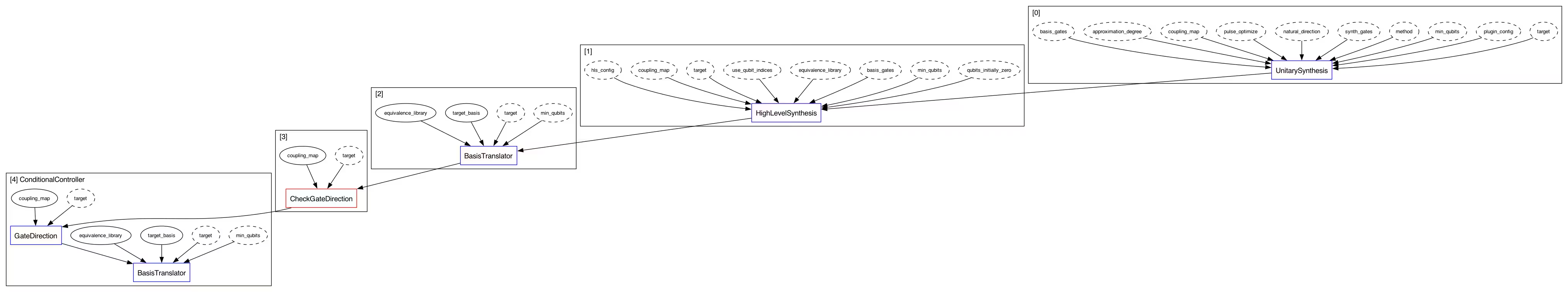
INFO:qiskit.passmanager.base_tasks:Pass: UnitarySynthesis - 0.03386 (ms)
INFO:qiskit.passmanager.base_tasks:Pass: HighLevelSynthesis - 0.02718 (ms)
INFO:qiskit.passmanager.base_tasks:Pass: BasisTranslator - 2.64192 (ms)
INFO:qiskit.passmanager.base_tasks:Pass: CheckGateDirection - 0.02217 (ms)
INFO:qiskit.passmanager.base_tasks:Pass: GateDirection - 0.36502 (ms)
INFO:qiskit.passmanager.base_tasks:Pass: BasisTranslator - 0.64778 (ms)

הערה: לא תמיד ניתן להריץ כל שלב בנפרד (כיוון שחלקם צריכים לשאת מידע משלב קודם).

3.4 שלב האופטימיזציה

השלב הדיפולטי האחרון בצינור הוא האופטימיזציה. לאחר שהטמענו את ה-Circuit לתוך ה-Backend, ה-Circuit התרחב מאוד. רוב ההתרחבות נובעת מחוסר יעילות ביחסי השקילות מתרגום הבסיס והכנסת החלפות. שלב האופטימיזציה מנסה למזער את הגודל והעומק של ה-Circuit. הוא מריץ סדרה של פאסים בלולאת do while loop until it reaches a steady output.

# pm.pre_optimization.draw()
pm.optimization.draw()

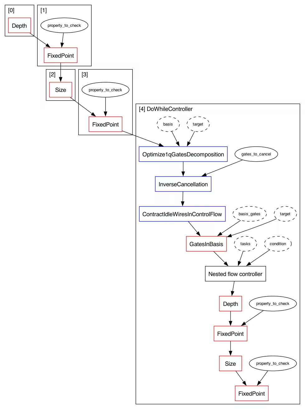
logger = logging.getLogger()
logger.setLevel("INFO")
opt_out = pm.optimization.run(basis_out)

INFO:qiskit.passmanager.base_tasks:Pass: Depth - 0.30112 (ms)
INFO:qiskit.passmanager.base_tasks:Pass: FixedPoint - 0.03195 (ms)
INFO:qiskit.passmanager.base_tasks:Pass: Size - 0.01216 (ms)
INFO:qiskit.passmanager.base_tasks:Pass: FixedPoint - 0.01001 (ms)
INFO:qiskit.passmanager.base_tasks:Pass: Optimize1qGatesDecomposition - 0.63729 (ms)
INFO:qiskit.passmanager.base_tasks:Pass: InverseCancellation - 0.41723 (ms)
INFO:qiskit.passmanager.base_tasks:Pass: ContractIdleWiresInControlFlow - 0.01192 (ms)
INFO:qiskit.passmanager.base_tasks:Pass: GatesInBasis - 0.05484 (ms)
INFO:qiskit.passmanager.base_tasks:Pass: Depth - 0.08583 (ms)
INFO:qiskit.passmanager.base_tasks:Pass: FixedPoint - 0.20599 (ms)
INFO:qiskit.passmanager.base_tasks:Pass: Size - 0.00787 (ms)
INFO:qiskit.passmanager.base_tasks:Pass: FixedPoint - 0.00715 (ms)
INFO:qiskit.passmanager.base_tasks:Pass: Optimize1qGatesDecomposition - 0.16809 (ms)
INFO:qiskit.passmanager.base_tasks:Pass: InverseCancellation - 0.17190 (ms)
INFO:qiskit.passmanager.base_tasks:Pass: ContractIdleWiresInControlFlow - 0.00691 (ms)
INFO:qiskit.passmanager.base_tasks:Pass: GatesInBasis - 0.02408 (ms)
INFO:qiskit.passmanager.base_tasks:Pass: Depth - 0.04935 (ms)
INFO:qiskit.passmanager.base_tasks:Pass: FixedPoint - 0.00525 (ms)
INFO:qiskit.passmanager.base_tasks:Pass: Size - 0.00620 (ms)
INFO:qiskit.passmanager.base_tasks:Pass: FixedPoint - 0.00286 (ms)

opt_out.draw("mpl", idle_wires=False, fold=-1)

4. דוגמאות מעמיקות

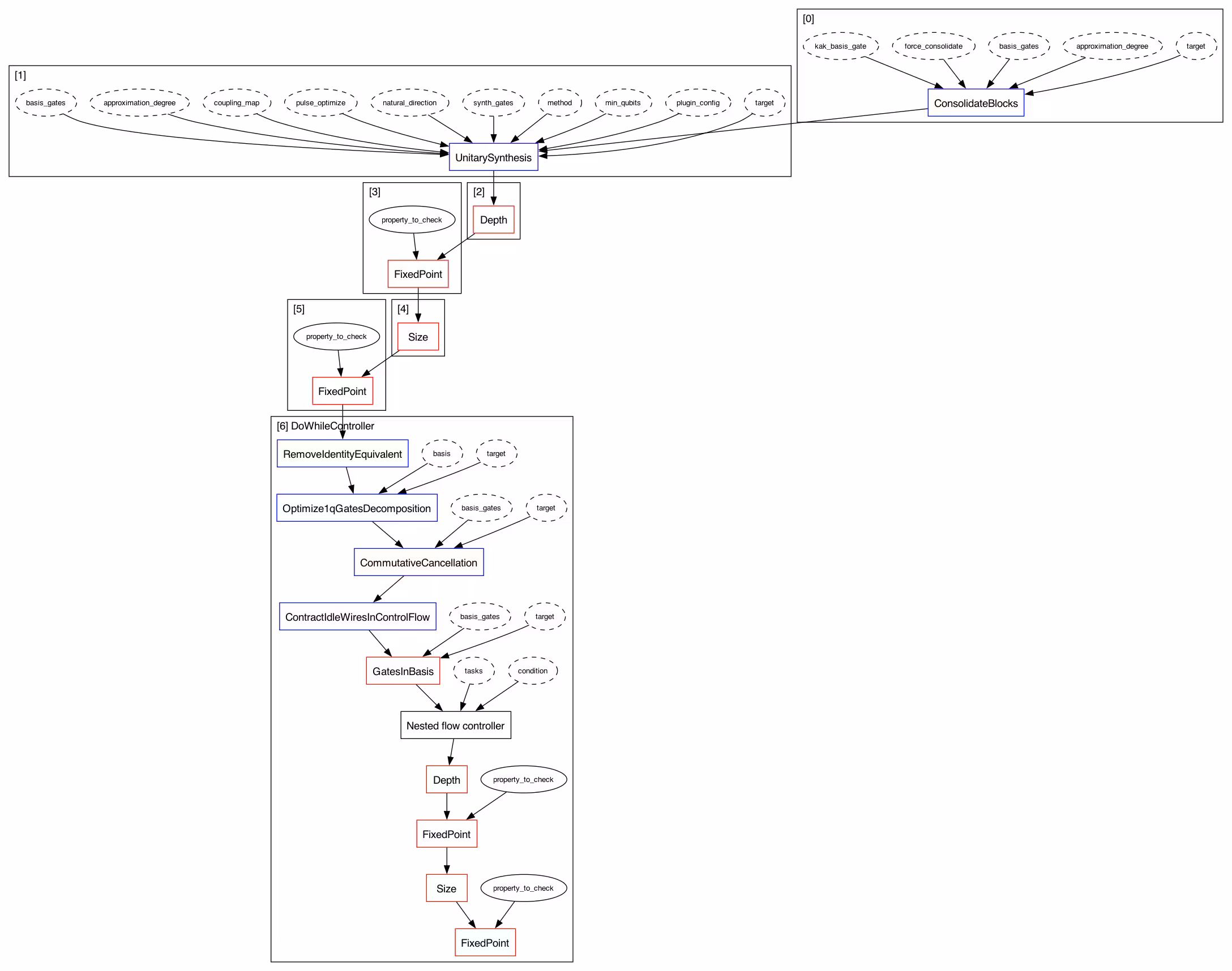
4.1 אופטימיזציית בלוקים של שני קיוביטים באמצעות סינתזת אוניטרי

ברמה 2 ו-3 יש לנו יותר passes (Collect2qBlocks, ConsolidateBlocks, UnitarySynthesis) לאופטימיזציה נוספת, כלומר אופטימיזציית בלוקים של שני קיוביטים. (השוו את זרימת שלב האופטימיזציה ברמה 2 לזו שמעל ברמה 1)

אופטימיזציית הבלוקים של שני קיוביטים מורכבת משני שלבים: איסוף וגיבוש בלוקי 2 קיוביטים, וסינתזת מטריצות אוניטריות של 2 קיוביטים.

pm2 = generate_preset_pass_manager(2, backend, seed_transpiler=42)
pm2.optimization.draw()

from qiskit.transpiler import PassManager
from qiskit.transpiler.passes import (
    Collect2qBlocks,
    ConsolidateBlocks,
    UnitarySynthesis,
)

# Collect 2q blocks and consolidate to unitary when we expect that we can reduce the 2q gate count for that unitary
consolidate_pm = PassManager(
    [
        Collect2qBlocks(),
        ConsolidateBlocks(target=backend.target),
    ]
)

display(basis_out.draw("mpl", idle_wires=False, fold=-1))

consolidated = consolidate_pm.run(basis_out)
consolidated.draw("mpl", idle_wires=False, fold=-1)

# Synthesize unitaries
UnitarySynthesis(target=backend.target)(consolidated).draw(
    "mpl", idle_wires=False, fold=-1
)

logger.setLevel("WARNING")

ראינו בחלק 2 שזרימת המהדר הקוונטי האמיתית אינה פשוטה כל כך, והיא בנויה מהרבה passes (משימות). זה נובע בעיקר מהצרכים ההנדסיים הנדרשים להבטחת ביצועים עבור מגוון רחב של מעגלי יישום ותחזוקה של התוכנה. ה-transpiler של Qiskit עובד טוב ברוב המקרים, אבל אם אתם רואים שה-Circuit שלכם לא ממוטב היטב על ידו — זו הזדמנות טובה לחקור אופטימיזציית Circuit ייעודית לאפליקציה שלכם, כפי שמוצג בחלק 1. טכנולוגיית ה-transpiler מתפתחת כל הזמן, ותרומת המחקר והפיתוח שלכם מוזמנת.

from qiskit.circuit import QuantumCircuit
from qiskit_ibm_runtime import QiskitRuntimeService, Sampler

service = QiskitRuntimeService()
backend = service.backend("ibm_brisbane")
sampler = Sampler(backend)

circ = QuantumCircuit(3)
circ.ccx(0, 1, 2)
circ.measure_all()
circ.draw("mpl")

sampler.run([circ])  # IBMInputValueError will be raised

4.2 אופטימיזציית Circuit חשובה

נתחיל בהשוואת תוצאות הרצת מעגלי הכנת מצב GHZ בן 5 קיוביטים ($\frac{1}{\sqrt{2}} \left( |00000\rangle + |11111\rangle \right)$) עם ובלי אופטימיזציה.

from qiskit.circuit import QuantumCircuit
from qiskit.transpiler.preset_passmanagers import generate_preset_pass_manager
from qiskit_ibm_runtime import QiskitRuntimeService, Sampler

service = QiskitRuntimeService()

# backend = service.backend('ibm_brisbane')
backend = service.least_busy(
    operational=True, simulator=False, min_num_qubits=127
)  # Eagle
backend

נתחיל עם Circuit GHZ שסונתז בצורה פשוטה כך:

num_qubits = 5

ghz_circ = QuantumCircuit(num_qubits)
ghz_circ.h(0)
[ghz_circ.cx(0, i) for i in range(1, num_qubits)]
ghz_circ.measure_all()
ghz_circ.draw("mpl")

אנחנו מבצעים transpile ל-Circuit בלי אופטימיזציה (optimization_level=0) ועם אופטימיזציה (optimization_level=2). כפי שניתן לראות, יש הבדל גדול באורך ה-Circuit לאחר ה-transpile.

pm0 = generate_preset_pass_manager(
    optimization_level=0, backend=backend, seed_transpiler=777
)
pm2 = generate_preset_pass_manager(
    optimization_level=2, backend=backend, seed_transpiler=777
)
circ0 = pm0.run(ghz_circ)
circ2 = pm2.run(ghz_circ)
print("optimization_level=0:")
display(circ0.draw("mpl", idle_wires=False, fold=-1))
print("optimization_level=2:")
display(circ2.draw("mpl", idle_wires=False, fold=-1))

optimization_level=0:

optimization_level=2:

# run the circuits
sampler = Sampler(backend)
job = sampler.run([circ0, circ2], shots=10000)
job_id = job.job_id()
print(f"Job ID: {job_id}")

Job ID: d13rnnemya70008ek1zg

# REPLACE WITH YOUR OWN JOB IDS
job = service.job(job_id)

# get results
result = job.result()
unoptimized_result = result[0].data.meas.get_counts()
optimized_result = result[1].data.meas.get_counts()

from qiskit.visualization import plot_histogram

# plot
sim_result = {"0" * 5: 0.5, "1" * 5: 0.5}
plot_histogram(
    [result for result in [sim_result, unoptimized_result, optimized_result]],
    bar_labels=False,
    legend=[
        "ideal",
        "no optimization",
        "with optimization",
    ],
)

4.3 סינתזת Circuit חשובה

כעת נשווה את תוצאות הרצת שני מעגלי הכנת מצב GHZ בן 5 קיוביטים ($\frac{1}{\sqrt{2}} \left( |00000\rangle + |11111\rangle \right)$) שסונתזו בצורות שונות.

# Original GHZ circuit (naive synthesis)
ghz_circ.draw("mpl")

# A better GHZ circuit (smarter synthesis), you learned in a previous lecture
ghz_circ2 = QuantumCircuit(5)
ghz_circ2.h(2)
ghz_circ2.cx(2, 1)
ghz_circ2.cx(2, 3)
ghz_circ2.cx(1, 0)
ghz_circ2.cx(3, 4)
ghz_circ2.measure_all()
ghz_circ2.draw("mpl")

circ_org = pm2.run(ghz_circ)
circ_new = pm2.run(ghz_circ2)
print("original synthesis:")
display(circ_org.draw("mpl", idle_wires=False, fold=-1))
print("new synthesis:")
display(circ_new.draw("mpl", idle_wires=False, fold=-1))

original synthesis:

new synthesis:

# run the circuits
sampler = Sampler(backend)
job = sampler.run([circ_org, circ_new], shots=10000)
job_id = job.job_id()
print(f"Job ID: {job_id}")

Job ID: d13rp283grvg008j12fg

# REPLACE WITH YOUR OWN JOB IDS
job = service.job(job_id)

# get results
result = job.result()
synthesis_org_result = result[0].data.meas.get_counts()
synthesis_new_result = result[1].data.meas.get_counts()

# plot
sim_result = {"0" * 5: 0.5, "1" * 5: 0.5}
plot_histogram(
    [result for result in [sim_result, synthesis_org_result, synthesis_new_result]],
    bar_labels=False,
    legend=[
        "ideal",
        "synthesis_org",
        "synthesis_new",
    ],
)

4.4 פירוק שערים כלליים של קיוביט אחד

from qiskit import QuantumCircuit, transpile
from qiskit.circuit import Parameter
from qiskit.circuit.library.standard_gates import UGate

phi, theta, lam = Parameter("φ"), Parameter("θ"), Parameter("λ")

qc = QuantumCircuit(1)
qc.append(UGate(theta, phi, lam), [0])
qc.draw(output="mpl")

transpile(qc, basis_gates=["rz", "sx"]).draw(output="mpl")

4.5 אופטימיזציית בלוק של קיוביט אחד

from qiskit import QuantumCircuit

qc = QuantumCircuit(1)
qc.x(0)
qc.y(0)
qc.z(0)
qc.rx(1.23, 0)
qc.ry(1.23, 0)
qc.rz(1.23, 0)
qc.h(0)
qc.s(0)
qc.t(0)
qc.sx(0)
qc.sdg(0)
qc.tdg(0)
qc.draw(output="mpl")

from qiskit.quantum_info import Operator

Operator(qc)

Operator([[ 0.45292511-0.57266982j, -0.66852684-0.14135058j],
          [ 0.14135058+0.66852684j, -0.57266982+0.45292511j]],
         input_dims=(2,), output_dims=(2,))

from qiskit import transpile

qc_opt = transpile(qc, basis_gates=["rz", "sx"])
qc_opt.draw(output="mpl")

Operator(qc_opt)

Operator([[ 0.45292511-0.57266982j, -0.66852684-0.14135058j],
          [ 0.14135058+0.66852684j, -0.57266982+0.45292511j]],
         input_dims=(2,), output_dims=(2,))

Operator(qc).equiv(Operator(qc_opt))

True

4.6 פירוק Toffoli

qc = QuantumCircuit(3)
qc.ccx(0, 1, 2)
qc.draw(output="mpl")

from qiskit import QuantumCircuit, transpile

qc = QuantumCircuit(3)
qc.ccx(0, 1, 2)
qc = transpile(qc, basis_gates=["rz", "sx", "cx"])
qc.draw(output="mpl")

4.7 פירוק שער CU

from qiskit.circuit.library.standard_gates import CUGate

phi, theta, lam, gamma = Parameter("φ"), Parameter("θ"), Parameter("λ"), Parameter("γ")
qc = QuantumCircuit(2)
# qc.cu(theta, phi, lam, gamma, 0, 1)
qc.append(CUGate(theta, phi, lam, gamma), [0, 1])
qc.draw(output="mpl")

from qiskit.circuit.library.standard_gates import CUGate

phi, theta, lam, gamma = Parameter("φ"), Parameter("θ"), Parameter("λ"), Parameter("γ")
qc = QuantumCircuit(2)
qc.append(CUGate(theta, phi, lam, gamma), [0, 1])
qc = transpile(qc, basis_gates=["rz", "sx", "cx"])
qc.draw(output="mpl")

4.8 CX, ECR, CZ שקולים עד כדי Cliffordים מקומיים

שימו לב ש-$H$ (Hadamard), $S$ (סיבוב Z ב-$\pi/2$), $S^\dagger$ (סיבוב Z ב-$-\pi/2$), $X$ (פאולי X) הם כולם שערי Clifford.

qc = QuantumCircuit(2)
qc.cx(0, 1)
qc.draw(output="mpl", style="bw")

qc = QuantumCircuit(2)
qc.cx(0, 1)
transpile(qc, basis_gates=["x", "s", "h", "sdg", "ecr"]).draw(output="mpl", style="bw")

qc = QuantumCircuit(2)
qc.cx(0, 1)
transpile(qc, basis_gates=["h", "cz"]).draw(output="mpl", style="bw")

שימוש בשערי הבסיס של קיוביט אחד של backend IBM: "rz", "sx" ו-"x".

qc = QuantumCircuit(2)
qc.cx(0, 1)
transpile(qc, basis_gates=["rz", "sx", "x", "ecr"]).draw(output="mpl", style="bw")

qc = QuantumCircuit(2)
qc.cx(0, 1)
transpile(qc, basis_gates=["rz", "sx", "x", "cz"]).draw(output="mpl", style="bw")

# Check Qiskit version
import qiskit

qiskit.__version__

'2.0.2'