מימוש ב-Qiskit

בשיעור זה נממש כמה מהרעיונות מהשיעור על שזירה בפעולה, תוך שימוש ב-Qiskit.

# Added by doQumentation — installs the packages this notebook needs if they are missing
import importlib.util

_needed = {"qiskit": "qiskit", "qiskit_aer": "qiskit-aer"}
_missing = [pip for module, pip in _needed.items()
            if importlib.util.find_spec(module) is None]
# One at a time, so a package that fails to install does not block the others
for _pip in _missing:
    %pip install -q {_pip}
if not _missing:
    print("\u2713 All required packages are installed")

from qiskit import __version__

print(__version__)

2.1.1

from qiskit import QuantumCircuit, QuantumRegister, ClassicalRegister
from qiskit_aer import AerSimulator
from qiskit.visualization import plot_histogram, array_to_latex
from qiskit.result import marginal_distribution
from qiskit.circuit.library import UGate
from math import pi
import random

הנה מימוש של פרוטוקול הטלפורטציה באמצעות Circuit קוונטי.

qubit = QuantumRegister(1, "Q")
ebit0 = QuantumRegister(1, "A")
ebit1 = QuantumRegister(1, "B")
a = ClassicalRegister(1, "a")
b = ClassicalRegister(1, "b")

protocol = QuantumCircuit(qubit, ebit0, ebit1, a, b)

# Prepare ebit used for teleportation
protocol.h(ebit0)
protocol.cx(ebit0, ebit1)
protocol.barrier()

# Alice's operations
protocol.cx(qubit, ebit0)
protocol.h(qubit)
protocol.barrier()

# Alice measures and sends classical bits to Bob
protocol.measure(ebit0, a)
protocol.measure(qubit, b)
protocol.barrier()

# Bob uses the classical bits to conditionally apply gates
with protocol.if_test((a, 1)):
    protocol.x(ebit1)
with protocol.if_test((b, 1)):
    protocol.z(ebit1)

display(protocol.draw(output="mpl"))

ה-Circuit משתמש בכמה תכונות של Qiskit שטרם ראינו בשיעורים קודמים, כולל הפונקציות barrier ו-if_test. הפונקציה barrier יוצרת הפרדה ויזואלית שהופכת את תרשים ה-Circuit לקריא יותר, וגם מונעת מ-Qiskit לבצע פישוטים ואופטימיזציות שונות דרך ה-barrier בזמן הידור כשה-Circuit רץ על חומרה אמיתית. הפונקציה if_test מפעילה פעולה באופן מותנה בהתאם לביט קלאסי או רגיסטר.

ה-Circuit מאתחל תחילה את $(\mathsf{A},\mathsf{B})$ למצב $\vert \phi^+\rangle$ (שאינו חלק מהפרוטוקול עצמו), ולאחר מכן מגיעות פעולות אליס, אחר כך המדידות שלה, ולבסוף פעולות בוב. כדי לבדוק שהפרוטוקול עובד נכון, נפעיל Gate של qubit בודד שנוצר באקראי על מצב $\vert 0\rangle$ המאותחל של $\mathsf{Q}$, כדי לקבל וקטור מצב קוונטי אקראי שיועבר בטלפורטציה. על ידי הפעלת ההופכי (כלומר הטרנספוז המצומד) של אותו Gate על $\mathsf{B}$ לאחר הרצת הפרוטוקול, נוכל לאמת שהמצב אכן עבר בטלפורטציה על ידי מדידה שמראה שהוא חזר למצב $\vert 0\rangle$.

ראשית נבחר באקראי Gate של qubit אוניטרי.

random_gate = UGate(
    theta=random.random() * 2 * pi,
    phi=random.random() * 2 * pi,
    lam=random.random() * 2 * pi,
)

display(array_to_latex(random_gate.to_matrix()))

$$\begin{bmatrix} 0.9897212158 & -0.0195080103 - 0.141673401 i \\ 0.0603319186 + 0.1296609988 i & -0.8319925233 + 0.5360378028 i \\ \end{bmatrix}$$

כעת ניצור Circuit בדיקה חדש שמפעיל תחילה את ה-Gate האקראי שלנו על $\mathsf{Q}$, לאחר מכן מריץ את Circuit הטלפורטציה, ולבסוף מפעיל את ההופכי של ה-Gate האקראי על ה-Qubit $\mathsf{B}$ ומודד. התוצאה צריכה להיות $0$ בוודאות.

# Create a new circuit including the same bits and qubits used in the
# teleportation protocol.

test = QuantumCircuit(qubit, ebit0, ebit1, a, b)

# Start with the randomly selected gate on Q

test.append(random_gate, qubit)
test.barrier()

# Append the entire teleportation protocol from above.

test = test.compose(protocol)
test.barrier()

# Finally, apply the inverse of the random unitary to B and measure.

test.append(random_gate.inverse(), ebit1)
result = ClassicalRegister(1, "Result")
test.add_register(result)
test.measure(ebit1, result)

display(test.draw(output="mpl"))

לבסוף, בואו נריץ את סימולטור Aer על ה-Circuit הזה ונציג היסטוגרמה של הפלטים. נראה את הסטטיסטיקות עבור שלושת הביטים הקלאסיים: הביט התחתון/השמאלי ביותר צריך תמיד להיות $0$, מה שמצביע על כך שה-Qubit $\mathsf{Q}$ עבר בהצלחה בטלפורטציה אל $\mathsf{B}$, בעוד ששני הביטים האחרים אמורים להיות אחידים פחות או יותר.

result = AerSimulator().run(test).result()
statistics = result.get_counts()
display(plot_histogram(statistics))

אפשר גם לסנן את הסטטיסטיקות כדי להתמקד אך ורק ב-Qubit של תוצאת הבדיקה, אם רוצים, כך:

filtered_statistics = marginal_distribution(statistics, [2])
display(plot_histogram(filtered_statistics))

קידוד על-צפוף

קידוד על-צפוף הוא פרוטוקול שמשיג, במובן מסוים, מטרה משלימה לטלפורטציה. במקום לאפשר העברה של qubit אחד תוך שימוש בשני ביטים קלאסיים של תקשורת (במחיר של e-bit אחד של שזירה), הוא מאפשר העברה של שני ביטים קלאסיים תוך שימוש ב-Qubit אחד של תקשורת קוונטית (שוב, במחיר של e-bit אחד של שזירה).

בפירוט רב יותר, יש לנו שולח (אליס) ומקבל (בוב) שחולקים e-bit אחד של שזירה. לפי המוסכמות של השיעור, פירוש הדבר הוא שאליס מחזיקה qubit $\mathsf{A}$, בוב מחזיק qubit $\mathsf{B}$, ויחד הזוג $(\mathsf{A},\mathsf{B})$ נמצא במצב $\vert\phi^+\rangle$. אליס רוצה להעביר לבוב שני ביטים קלאסיים, שנסמן אותם $c$ ו-$d$, והיא תעשה זאת על ידי שליחת qubit אחד.

אפשר לראות בהישג הזה הישג פחות מעניין מזה שמשיגה הטלפורטציה. שליחת qubits צפויה להיות קשה בהרבה משליחת ביטים קלאסיים בעתיד הנראה לעין, כך שהחלפה של qubit אחד של תקשורת קוונטית בשני ביטים של תקשורת קלאסית, במחיר של e-bit לא פחות, בקושי נראית כדאית. אולם, זה לא אומר שקידוד על-צפוף אינו מעניין, כי הוא בהחלט כן.

בהתאם לנושא השיעור, סיבה אחת לכך שקידוד על-צפוף מעניין היא שהוא מדגים שימוש קונקרטי ו(בהקשר של תורת המידע) מרשים למדי בשזירה. משפט מפורסם בתורת המידע הקוונטי, הידוע כמשפט הולבו, גורר שללא שימוש במצב שזור משותף, אי אפשר להעביר יותר מביט קלאסי אחד על ידי שליחת qubit בודד. (משפט הולבו הוא כללי יותר מכך. הניסוח המדויק שלו טכני ומצריך הסבר, אבל זו אחת המסקנות שנובעות ממנו.) כך, דרך קידוד על-צפוף, שזירה משותפת למעשה מאפשרת הכפלה של קיבולת נשיאת המידע הקלאסי בשליחת qubits.

פרוטוקול

דיאגרמת המעגל הקוונטי הבאה מתארת את פרוטוקול הקידוד העל-צפוף:

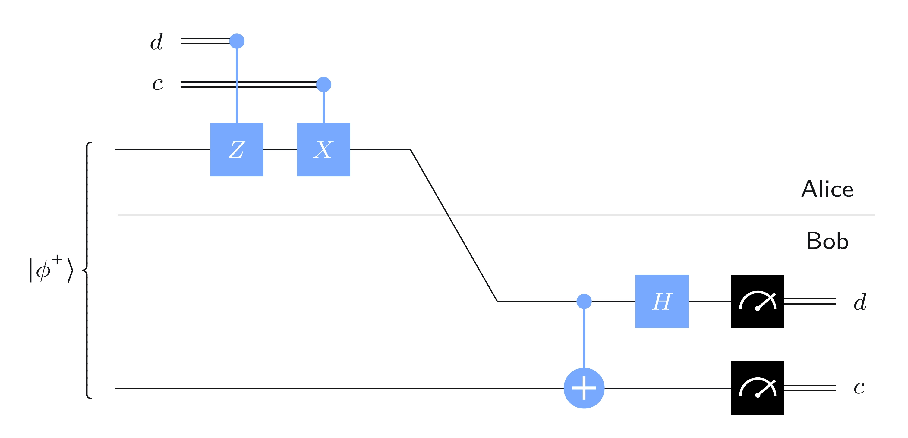
הנה מה שאליס עושה, בלשון פשוטה:

1. אם $d=1$, אליס מפעילה Gate מסוג $Z$ על ה-Qubit שלה $\mathsf{A}$ (ואם $d=0$ היא לא עושה כלום).

2. אם $c=1$, אליס מפעילה Gate מסוג $X$ על ה-Qubit שלה $\mathsf{A}$ (ואם $c=0$ היא לא עושה כלום).

לאחר מכן אליס שולחת את ה-Qubit שלה $\mathsf{A}$ לבוב.

מה שבוב עושה כשהוא מקבל את ה-Qubit $\mathsf{A}$ הוא קודם כל להפעיל Gate מסוג controlled-NOT, כשהבקרה היא $\mathsf{A}$ והמטרה היא $\mathsf{B}$, ואז הוא מפעיל Gate מסוג Hadamard על $\mathsf{A}$. לאחר מכן הוא מודד את $\mathsf{B}$ כדי לקבל את $c$ ואת $\mathsf{A}$ כדי לקבל את $d$, ובשני המקרים בבסיס הסטנדרטי.

ניתוח

הרעיון מאחורי פרוטוקול זה פשוט: אליס בעצם בוחרת איזה מצב Bell היא רוצה לשתף עם בוב, היא שולחת לבוב את ה-Qubit שלה, ובוב מודד כדי לקבוע איזה מצב Bell אליס בחרה.

כלומר, הם משתפים בהתחלה את $\vert\phi^+\rangle,$ ובהתאם לביטים $c$ ו-$d,$ אליס או משאירה את המצב כמו שהוא או משנה אותו לאחד ממצבי Bell האחרים על ידי הפעלת $\mathbb{I},$ $X,$ $Z,$ או $XZ$ על ה-Qubit שלה $\mathsf{A}.$

$$\begin{aligned} (\mathbb{I} \otimes \mathbb{I}) \vert \phi^+ \rangle & = \vert \phi^+\rangle \\ (\mathbb{I} \otimes Z) \vert \phi^+ \rangle & = \vert \phi^-\rangle \\ (\mathbb{I} \otimes X) \vert \phi^+ \rangle & = \vert \psi^+\rangle \\ (\mathbb{I} \otimes XZ) \vert \phi^+ \rangle & = \vert \psi^-\rangle \end{aligned}$$

הפעולות של בוב גורמות לאפקטים הבאים על ארבעת מצבי Bell:

$$\begin{aligned} \vert \phi^+\rangle & \mapsto \vert 00\rangle\\ \vert \phi^-\rangle & \mapsto \vert 01\rangle\\ \vert \psi^+\rangle & \mapsto \vert 10\rangle\\ \vert \psi^-\rangle & \mapsto -\vert 11\rangle\\ \end{aligned}$$

אפשר לאמת זאת ישירות, על ידי חישוב תוצאות הפעולות של בוב על מצבים אלה אחד אחד.

כך, כאשר בוב מבצע את המדידות שלו, הוא מסוגל לקבוע איזה מצב Bell אליס בחרה. כדי לאמת שהפרוטוקול עובד נכון מספיק לבדוק כל מקרה:

• אם $cd = 00$, אז המצב של $(\mathsf{B},\mathsf{A})$ כאשר בוב מקבל את $\mathsf{A}$ הוא $\vert \phi^+\rangle$. הוא הופך מצב זה ל-$\vert 00\rangle$ ומקבל $cd = 00$.

• אם $cd = 01$, אז המצב של $(\mathsf{B},\mathsf{A})$ כאשר בוב מקבל את $\mathsf{A}$ הוא $\vert \phi^-\rangle$. הוא הופך מצב זה ל-$\vert 01\rangle$ ומקבל $cd = 01$.

• אם $cd = 10$, אז המצב של $(\mathsf{B},\mathsf{A})$ כאשר בוב מקבל את $\mathsf{A}$ הוא $\vert \psi^+\rangle$. הוא הופך מצב זה ל-$\vert 10\rangle$ ומקבל $cd = 10$.

• אם $cd = 11$, אז המצב של $(\mathsf{B},\mathsf{A})$ כאשר בוב מקבל את $\mathsf{A}$ הוא $\vert \psi^-\rangle$. הוא הופך מצב זה ל-$-\vert 11\rangle$ ומקבל $cd = 11$. (גורם הפאזה של מינוס אחד אינו משפיע כאן.)

מימוש קידוד על-צפוף

הנה מימוש פשוט של קידוד על-צפוף שבו אנחנו מגדירים את ה-Circuit עצמו בהתאם לביטים שרוצים לשדר. ראשית נבחר שני ביטים לשידור. (בהמשך נבחר אותם אקראית, אבל לעכשיו פשוט נעשה בחירה שרירותית.)

c = "1"
d = "0"

עכשיו נבנה את ה-Circuit בהתאם. כאן נאפשר ל-Qiskit להשתמש בשמות ברירת המחדל עבור ה-Qubits: $\mathsf{q}_0$ עבור ה-Qubit העליון ו-$\mathsf{q}_1$ עבור התחתון.

protocol = QuantumCircuit(2)

# Prepare ebit used for superdense coding
protocol.h(0)
protocol.cx(0, 1)
protocol.barrier()

# Alice's operations
if d == "1":
    protocol.z(0)
if c == "1":
    protocol.x(0)
protocol.barrier()

# Bob's actions
protocol.cx(0, 1)
protocol.h(0)
protocol.measure_all()

display(protocol.draw(output="mpl"))

אין כאן הרבה חדש, פרט לפונקציה measure_all, שמודדת את כל ה-Qubits ומכניסה את התוצאות לרגיסטר קלאסי אחד (ולכן במקרה זה יהיו בו שני ביטים).

הרצת הסימולטור Aer מניבה את הפלט הצפוי.

result = AerSimulator().run(protocol).result()
statistics = result.get_counts()

for outcome, frequency in statistics.items():
    print(f"Measured {outcome} with frequency {frequency}")

display(plot_histogram(statistics))

Measured 10 with frequency 1024

עכשיו בואו נשתמש ב-Qubit נוסף כמחולל ביטים אקראיים — בעצם כדי להטיל מטבעות הוגנים. נשתמש בו לבחירה אקראית של $c$ ו-$d$, ואז נריץ את פרוטוקול הקידוד העל-צפוף.

rbg = QuantumRegister(1, "coin")
ebit0 = QuantumRegister(1, "A")
ebit1 = QuantumRegister(1, "B")

Alice_c = ClassicalRegister(1, "Alice c")
Alice_d = ClassicalRegister(1, "Alice d")

test = QuantumCircuit(rbg, ebit0, ebit1, Alice_d, Alice_c)

# Initialize the ebit
test.h(ebit0)
test.cx(ebit0, ebit1)
test.barrier()

# Use the 'coin' qubit twice to generate Alice's bits c and d.
test.h(rbg)
test.measure(rbg, Alice_c)
test.h(rbg)
test.measure(rbg, Alice_d)
test.barrier()

# Now the protocol runs, starting with Alice's actions, which depend
# on her bits.
with test.if_test((Alice_d, 1), label="Z"):
    test.z(ebit0)
with test.if_test((Alice_c, 1), label="X"):
    test.x(ebit0)
test.barrier()

# Bob's actions
test.cx(ebit0, ebit1)
test.h(ebit0)
test.barrier()

Bob_c = ClassicalRegister(1, "Bob c")
Bob_d = ClassicalRegister(1, "Bob d")
test.add_register(Bob_d)
test.add_register(Bob_c)
test.measure(ebit0, Bob_d)
test.measure(ebit1, Bob_c)

display(test.draw(output="mpl"))

הרצת הסימולטור Aer מציגה את התוצאות: הביטים הקלאסיים של אליס ובוב תמיד מסכימים.

result = AerSimulator().run(test).result()
statistics = result.get_counts()
display(plot_histogram(statistics))

מימוש ב-Qiskit

אנחנו יכולים לממש את משחק CHSH, יחד עם האסטרטגיה הקוונטית שהוגדרה לעיל, ב-Qiskit כך.

ראשית, הנה הגדרת המשחק עצמו, שמאפשרת לחבר כל אסטרטגיה שרירותית כארגומנט.

def chsh_game(strategy):
    # This function runs the CHSH game, using the strategy (a function
    # from two bits to two bits), returning 1 for a win and 0 for a loss.

    # Choose x and y randomly
    x, y = random.randint(0, 1), random.randint(0, 1)

    # Use the strategy to determine a and b
    a, b = strategy(x, y)

    # Decide if the strategy wins or loses
    if (a != b) == (x & y):
        return 1  # Win
    return 0  # Lose

עכשיו ניצור פונקציה שמפיקה Circuit בהתאם לשאלות עבור אליס ובוב. נשאיר לקיוביטים את שמות ברירת המחדל שלהם לפשטות, ונשתמש ב-Gate המובנה $R_y(\theta)$ עבור פעולות אליס ובוב.

def chsh_circuit(x, y):
    # This function creates a `QuantumCircuit` implementing the quantum
    # strategy described above (including the e-bit preparation).

    qc = QuantumCircuit(2, 2)

    # Prepare an e-bit
    qc.h(0)
    qc.cx(0, 1)
    qc.barrier()

    # Alice's actions
    if x == 0:
        qc.ry(0, 0)
    else:
        qc.ry(-pi / 2, 0)
    qc.measure(0, 0)

    # Bob's actions
    if y == 0:
        qc.ry(-pi / 4, 1)
    else:
        qc.ry(pi / 4, 1)
    qc.measure(1, 1)

    return qc

הנה ארבעת ה-Circuits האפשריים, בהתאם לשאלות שנשאלות.

# Draw the four possible circuits

print("(x,y) = (0,0)")
display(chsh_circuit(0, 0).draw(output="mpl"))

print("(x,y) = (0,1)")
display(chsh_circuit(0, 1).draw(output="mpl"))

print("(x,y) = (1,0)")
display(chsh_circuit(1, 0).draw(output="mpl"))

print("(x,y) = (1,1)")
display(chsh_circuit(1, 1).draw(output="mpl"))

(x,y) = (0,0)

(x,y) = (0,1)

(x,y) = (1,0)

(x,y) = (1,1)

עכשיו ניצור עבודה באמצעות סימולטור Aer שמריצה את ה-Circuit פעם אחת עבור זוג קלט נתון $(x,y)$.

def quantum_strategy(x, y):
    # This function runs the appropriate quantum circuit defined above
    # one time and returns the measurement results

    # Setting `shots=1` to run the circuit once
    result = AerSimulator().run(chsh_circuit(x, y), shots=1).result()
    statistics = result.get_counts()

    # Determine the output bits and return them
    bits = list(statistics.keys())[0]
    a, b = bits[0], bits[1]
    return a, b

לבסוף, נשחק את המשחק 1000 פעמים ונחשב את שיעור הניצחונות של האסטרטגיה.

NUM_GAMES = 1000
TOTAL_SCORE = 0

for _ in range(NUM_GAMES):
    TOTAL_SCORE += chsh_game(quantum_strategy)

print("Fraction of games won:", TOTAL_SCORE / NUM_GAMES)

Fraction of games won: 0.867

אנחנו יכולים גם להגדיר אסטרטגיה קלאסית ולראות עד כמה היא עובדת. זו רק אסטרטגיה אחת — אחרות ניתנות לבדיקה על ידי שינוי הקוד — אבל היא נמצאת בין האסטרטגיות הקלאסיות האופטימליות.

def classical_strategy(x, y):
    # This function implements just one example of an optimal classical
    # strategy for the CHSH game. Other classical strategies can be
    # implemented by changing the bit values assigned to a and b.

    # Alice's answer
    if x == 0:
        a = 0
    elif x == 1:
        a = 1

    # Bob's answer
    if y == 0:
        b = 1
    elif y == 1:
        b = 0

    return a, b

שוב, נשחק את המשחק 1000 פעמים כדי לראות עד כמה היא עובדת.

NUM_GAMES = 1000
TOTAL_SCORE = 0

for _ in range(NUM_GAMES):
    TOTAL_SCORE += chsh_game(classical_strategy)

print("Fraction of games won:", TOTAL_SCORE / NUM_GAMES)

Fraction of games won: 0.747

למרות שיש מעורבות אקראיות, לא סביר שהסטטיסטיקה תסטה יותר מדי לאחר 1000 הרצות. האסטרטגיה הקוונטית מנצחת בכ-85% מהזמן, בעוד שאסטרטגיה קלאסית לא יכולה לנצח ביותר מכ-75% מהזמן.