Shadow tomography של מצב Greenberger-Horne-Zeilinger

הערכת שימוש: פחות מ-10 שניות על מעבד Heron r2 (הערה: זו הערכה בלבד. זמן הריצה שלכם עשוי להיות שונה.)

תוצאות למידה

• איך shadow tomography בונה צל קלאסי של מצב קוונטי, ולמה היא דורשת מספר מדידות קטן אקספוננציאלית בהשוואה לטומוגרפיה מלאה של המצב

• איך לממש shadow tomography מקומית של Pauli באמצעות Qiskit, כדי להעריך מגנטיזציות של qubit בודד, מתאמים דו-נקודתיים ומטריצות צפיפות מצומצמות של שני qubit

• איך להשתמש ב-qiskit-paulice לזיהוי שגיאות בתקורה נמוכה באמצעות קודי מרחב-זמן בניסוי חומרה בקנה מידה גדול

דרישות קדם

• מדידות

• טומוגרפיית מצב קוונטי

• זיהוי שגיאות באמצעות קודי מרחב-זמן

רקע

טומוגרפיה מלאה של מצב קוונטי של מערכת בת $N$ qubit דורשת מספר מדידות אקספוננציאלי כדי להעריך את כל $4^N -1$ הפרמטרים הבלתי תלויים של מטריצת הצפיפות. למשל, עבור מערכת של 50 qubit, התהליך הזה דורש בסדר גודל של $10^{30}$ shots, יותר ממיליארד פעמים מספר הכוכבים ביקום הנצפה. Shadow tomography [1] היא פרוטוקול של תורת האינפורמציה הקוונטית הבונה "צל קלאסי" של המצב הקוונטי, שממנו אפשר להעריך אובזרבלס מטרה באמצעות מספר shots שגדל באופן לוגריתמי במספר האובזרבלס ואינו תלוי בגודל המערכת $N$. זה הופך אותה לרלוונטית בתחומים רבים במחשוב קוונטי, ובהם הערכת אנרגיה, חישובי אנטרופיית הspecial-entanglement ופונקציות מתאם, הערכת קרנלים בלמידת מכונה קוונטית ועוד.

המדריך הזה מראה איך להשתמש ב-shadow tomography כדי להעריך אובזרבלס מקומיים, כמו המגנטיזציה של qubit בודד $\langle Z_i \rangle$ עבור qubit $i$, פונקציית המתאם הדו-נקודתית $\langle Z_i Z_j\rangle$ ומטריצת הצפיפות המצומצמת של שני qubit (2-RDM), של מצב Greenberger-Horne-Zeilinger (GHZ) השזור מאוד. תחילה המדריך ממחיש תהליך עבודה קטן של shadow tomography על מצב GHZ של 10 qubit באמצעות סימולציית statevector. לאחר מכן הוא מציג הדגמה של 100 qubit על חומרה קוונטית אמיתית.

פרוטוקול Shadow tomography

פרוטוקול ה-shadow tomography כולל את השלבים הבאים:

1. מפעילים אופרטור אוניטרי אקראי $U$, הנבחר מתוך אנסמבל אוניטרי, על המצב הקוונטי ההתחלתי.
2. מודדים את התוצאה בבסיס החישובי ומקבלים מחרוזת ביטים $\ket{b}$.
3. שומרים את התמונה הקלאסית, $\hat{\rho} = \mathcal{M}^{-1}(U^{\dagger}\ket{b}\bra{b}U)$, כאשר $\mathcal{M}^{-1}$ הוא ההופכי של ערוץ המדידה $\mathcal{M}(\rho)=\mathbb{E}[U^{\dagger}\ket{b}\bra{b}U]$.
4. חוזרים על התהליך $T$ פעמים, כאשר אוסף $T$ התמונות $\{\hat{\rho}_t\}$ יוצר צל קלאסי $S(\rho, T)$.
5. מעריכים את האובזרבל $o$ של האופרטור $O$ כ-$\frac{1}{T}\sum_{t=1}^{T}\text{Tr}(O\hat{\rho}_t)$.

גרסאות של Shadow tomography

בחירת האנסמבל האוניטרי, כלומר הבסיס, בשלב 1 של הפרוטוקול משפיעה על מורכבות הדגימה, על השונות של ההערכות ועל שלמות האינפורמציה של shadow tomography נתונה. בספרות נבחנו קבוצות אנסמבל רבות, וכל אחת מהן כרוכה בפשרות בין מורכבות ליעילות הערכת האובזרבלס. התכונות של הגרסאות הנפוצות ביותר מסוכמות בטבלה הבאה, אם כי הרשימה אינה ממצה.

גרסה	אנסמבל	מורכבות דגימה	עומק מעגל	אובזרבלס מתאימים
Pauli מקומי [1]	אופרטורי Pauli של qubit בודד $\{X, Y, Z\}$	$\mathcal{O}(3^k\text{log}M/\varepsilon^2)$	1	מקומיים/מעט גופים
Clifford גלובלי [1]	Clifford של $N$ qubit	$\mathcal{O}(\text{Tr}(O^2)\text{log}M/\varepsilon^2)$	$\mathcal{O}(N\text{log}N)$	דרגה נמוכה, פידליות
גאוסיאני פרמיוני [2], [3]	מעגלי matchgate	$\mathcal{O}(\binom{\mu}{k}\frac{1}{\varepsilon^2})$	$\mathcal{O}(N^2)$	פרמיוניים
shallow shadows [4], [5]	מעגלים רדודים	$\mathcal{O}(k2^k\text{log}M/\varepsilon^2)$	$\mathcal{O}(\text{log}N)$	לא מקומיים (ידידותיים לחומרה)

המונחים שבטבלה מוגדרים כך:

• "מורכבות דגימה" מתייחסת למספר המדידות הנדרש עבור גרסה נתונה של shadow tomography.

• "עומק מעגל" מתאר עד כמה יקר לממש את המדידות על חומרה קוונטית.

• $N$ הוא מספר ה-qubit.

• $k$ הוא המקומיות של האובזרבל (לדוגמה, ל-$\langle Z_i \rangle$ יש $k=1$ ול-$\langle Z_i Z_j\rangle$ יש $k=2$).

• $M$ הוא מספר האובזרבלס שיש להעריך בו-זמנית.

• $\varepsilon$ הוא סבולת השגיאה החיבורית.

• $\mu$ הוא מספר הפרמיונים.

אף שאנסמבל Pauli המקומי הוא הידידותי ביותר לחומרה, הוא משלם קנס מורכבות דגימה של $3^k$, מה שהופך אותו ללא מתאים להערכת תכונות לא מקומיות. באופן כללי יותר, החסם על מורכבות הדגימה של צל מקומי גדל כמו $4^k$, ומשתפר ל-$3^k$ במקרה המיוחד של אובזרבלס מכפלה טנזורית.

לעומת זאת, אף שאפשר להשתמש באנסמבל Clifford הגלובלי להערכת אובזרבלס לא מקומיים, עומק המעגל שלו אינו נוח. צללים גאוסיאניים פרמיוניים מועילים בסימולציות של פיזיקת גופים רבים, כימיה וחומרים, אך דורשים מעגלי matchgate, שעלולים לשאת תקורה משמעותית במכשירים כלליים מבוססי שערים.

ל-Shallow shadows יש עומק מעגל שבין Pauli המקומי ל-Clifford הגלובלי, מה שהופך אותה לגרסה מבטיחה מאוד ליישום מעשי, אם כי עדיין יש כמה שאלות פתוחות לגבי עומק המעגל האופטימלי עבור אובזרבל נתון.

ככל שחזית המחקר של shadow tomography ממשיכה להתרחב, חלק מהבעיות הרלוונטיות ביותר לטיפול כוללות בחירה אופטימלית של אנסמבל המדידה עבור קבוצת אובזרבלס מטרה, שיפור החסמים על מורכבות הדגימה, והרחבת הפרוטוקול לאובזרבלס המתפתחים בזמן. עם זאת, shadow tomography עדיין מהווה אחד מתהליכי העבודה המובילים להפקת מקסימום אינפורמציה קלאסית ממצב קוונטי באמצעות מספר מדידות מינימלי, מה שהופך אותה לאידיאלית לאפיון מצבים קוונטיים בקנה מידה שבו גם טומוגרפיה מלאה וגם סימולציה קלאסית אינן אפשריות.

אנסמבל Pauli המקומי

המדריך הזה משתמש בבסיס Pauli אקראי, כלומר בשערי Clifford של qubit בודד, כדי לאסוף צללים ולהעריך תכונות של מצב GHZ. שימו לב שמדידות Pauli הן בחירה מצוינת להערכת אובזרבלס מקומיים (כמו צפיפות ספין, פונקציות מתאם מקומיות וצפיפות הסתברות מיקום), אך לא של אובזרבלס גלובליים (כמו אנרגיה כוללת, תנע ומטען).

כאן נבחר באופן בלתי תלוי בסיס Pauli אקראי $\{X, Y, Z\}$ לכל qubit, מופעל סיבוב ה-qubit הבודד המתאים, ואחריו מדידה:

$$\begin{equation} U = U_0 \otimes U_1 \otimes \cdots \otimes U_{n-1}, U_q \in \{I, H, S^{\dagger}H\} \end{equation} \tag{1}$$

עבור האנסמבל הזה, ההופכי של ערוץ המדידה הוא:

$$\begin{equation} \hat{\rho}_q=3U_q^{\dagger}\ket{b_q}\bra{b_q}U_q - I \end{equation} \tag{2}$$

הגורם $3$ נובע מממוצע על שלושת בסיסי Pauli, שיוצר ערוץ דה-פולריזציה עם פרמטר $\frac{1}{3}$. האסטימטור המלא מתפרק אז למכפלה של אסטימטורים של qubit בודד. כפי שמוצג בטבלה, עבור $M$ אובזרבלס, כל אחד במקומיות $k$, מספר צללי Pauli הדרוש כדי להעריך את כל האובזרבלס בשגיאה חיבורית $\varepsilon$ בהסתברות גבוהה הוא $\mathcal{O}(\frac{3^k\text{log}(M)}{\varepsilon^2})$. גודל המערכת אינו משפיע על עלות המדידה כל עוד האובזרבלס נשארים מקומיים, ולכן אפשר להעריך מספר אקספוננציאלי של אובזרבלס בו-זמנית בעלות לוגריתמית בלבד.

Median of means

ממוצע פשוט על פני $T$ תמונות מקטין את השונות של הערכת shot בודד של אובזרבל כמו $\frac{1}{T}$, אך הוא רגיש לחריגים. אפשר להשתמש ב-median of means כדי לטפל בכך. התהליך כולל:

• חלוקת $T$ התמונות ל-$K$ קבוצות שוות גודל
• חישוב הממוצע בתוך כל קבוצה
• החזרת החציון של ממוצעי הקבוצות

המדריך הזה מבצע shadow tomography מקומית של Pauli כדי להעריך תכונות של מצב GHZ, תחילה בדוגמה מדומה של 10 qubit ולאחר מכן בניסוי חומרה של 100 qubit.

דרישות

לפני שמתחילים את המדריך הזה, ודאו שמותקן אצלכם:

• Qiskit SDK גרסה 2.0 ומעלה, עם תמיכה ב-visualization

• IBM Quantum Compute גרסה 0.28 ומעלה (pip install qiskit-ibm-runtime)

• Qiskit Paulice (pip install qiskit-paulice)

הגדרה

# Added by doQumentation — installs the packages this notebook needs if they are missing
import importlib.util

_needed = {"matplotlib": "matplotlib", "numpy": "numpy", "qiskit": "qiskit", "qiskit_ibm_runtime": "qiskit-ibm-runtime", "qiskit_paulice": "qiskit-paulice"}
_missing = [pip for module, pip in _needed.items()
            if importlib.util.find_spec(module) is None]
# One at a time, so a package that fails to install does not block the others
for _pip in _missing:
    %pip install -q {_pip}
if not _missing:
    print("\u2713 All required packages are installed")

import numpy as np
import matplotlib.pyplot as plt
from collections import deque, defaultdict
from qiskit import QuantumCircuit, ClassicalRegister
from qiskit.quantum_info import (
    Statevector,
    partial_trace,
    Operator,
    Pauli,
    SparsePauliOp,
)
from qiskit.transpiler import generate_preset_pass_manager
from qiskit_ibm_runtime import QiskitRuntimeService
from qiskit_ibm_runtime import SamplerV2 as Sampler
from qiskit_paulice.layout import get_low_overhead_ancillas

seed = 42  # for reproducibility
rng = np.random.default_rng(seed)

פונקציות העזר הבאות משמשות בדוגמת החומרה בקנה מידה גדול בהמשך המדריך:

• bad_cz, bad_readout, bad_coherence — שולפות את נתוני הכיול של ה-Backend כדי לזהות שערים, qubit וקשתות החורגים מספי שגיאה או קוהרנטיות, כך שאפשר להוציא אותם מה-layout של המעגל.

• parallel_ghz — בונה מעגל GHZ בגודל נתון באמצעות חיפוש לרוחב על מפת הצימוד, ומפזרת שכבות CNOT במקביל כדי למזער את עומק המעגל.

• weighted_coverage, active_wires, z_trace_backward — מחשבות איזה חלק ממשטח השגיאות של מעגל ה-GHZ מוגן על ידי קבוצה נתונה של בדיקות זוגיות מרחב-זמן, באמצעות טכניקת ההתפשטות לאחור מתוך [6].

• add_measurements — מוסיפה מדידות של qubit-ים של GHZ ושל qubit-ים של בדיקות לרגיסטרים קלאסיים נפרדים, כך שאפשר לבצע עליהם postselection באופן בלתי תלוי.

• build_shadow_circuits — מפיקה מעגל אחד לכל בסיס Pauli אקראי, באמצעות הוספת סיבובי qubit בודד המתאימים לפני המדידה.

• parse_hw_results_w_checks — מפרקת את הפלט של Sampler לשלשות (ghz_bits, check_bits, bases), אחת לכל shot.

• adapt_to_flat_bits, estimate_zz_nn_hw — ממפות את הביטים של רגיסטר ה-GHZ בחזרה למרחב האינדקסים של כל המכשיר ומחשבות את ההערכה של median-of-means עבור $\langle Z_i Z_{i+1}\rangle$.

def bad_cz(target, threshold: float = 0.01) -> list:
    "Return edges whose CZ error exceeds threshold."
    edges = []
    for edge in backend.target.build_coupling_map().get_edges():
        if (edge[1], edge[0]) not in edges:
            edges.append(edge)
    cz_errors = {edge: target["cz"][edge].error for edge in edges}
    worst = sorted(cz_errors.items(), key=lambda x: x[1], reverse=True)
    return [list(edge) for edge, error in worst if error > threshold]

def bad_readout(target, threshold: float = 0.01) -> list:
    "Return nodes whose measurement error exceeds threshold."
    meas_errors = {
        node: target["measure"][(node,)].error
        for node in range(backend.num_qubits)
    }
    worst = sorted(meas_errors.items(), key=lambda x: x[1], reverse=True)
    return [node for node, error in worst if error > threshold]

def bad_coherence(target, threshold: float = 60) -> list:
    "Return nodes whose T2 value is below threshold."
    t2s = {
        node: (target.qubit_properties[node].t2 or 0) * 1e6
        for node in range(backend.num_qubits)
    }
    return [
        node
        for node, val in sorted(t2s.items(), key=lambda x: x[1])
        if val < threshold
    ]

def parallel_ghz(
    root: int, num_qubits: int, backend, bad_edges: list, skip: list
) -> tuple:
    "Build a GHZ circuit of size num_qubits using BFS from root, one neighbor per layer."
    edges = [
        e
        for e in [list(e) for e in backend.coupling_map.get_edges()]
        if e not in bad_edges
        and [e[1], e[0]] not in bad_edges
        and e[0] not in skip
        and e[1] not in skip
    ]
    adj = defaultdict(list)
    for u, v in edges:
        adj[u].append(v)
        adj[v].append(u)

    qc = QuantumCircuit(backend.num_qubits)
    visited = [root]
    queue = deque([root])
    explored = defaultdict(set)
    layers = []
    qc.h(root)

    while queue and len(visited) < num_qubits:
        layer = []
        for node in list(queue):
            queue.popleft()
            unvisited = [
                nb
                for nb in adj[node]
                if nb not in visited and nb not in explored[node]
            ]
            if unvisited:
                nb = unvisited[0]
                visited.append(nb)
                queue.append(node)
                queue.append(nb)
                explored[node].add(nb)
                layer.append((node, nb))
                if len(visited) == num_qubits:
                    break
        if layer:
            layers.append(layer)
        else:
            break

    for layer in layers:
        for q1, q2 in layer:
            qc.cx(q1, q2)
        qc.barrier()

    return qc, visited, layers

def weighted_coverage(
    layers: list, parities: list, w_idle: float = 0.2, w_gate: float = 0.8
) -> float:
    "Compute weighted fraction of wires covered by at least one parity check."
    wires = active_wires(layers)
    covered_by_any = {n_layer: set() for n_layer in range(len(layers))}
    for parity in parities:
        for n_layer, qs in z_trace_backward(layers, parity).items():
            covered_by_any[n_layer] |= qs
    covered_weight = total_weight = 0
    for n_layer in range(len(layers)):
        idle = wires[n_layer]["idle"]
        gate = wires[n_layer]["gate"]
        total_weight += w_idle * len(idle) + w_gate * len(gate)
        covered_weight += w_idle * len(
            covered_by_any[n_layer] & idle
        ) + w_gate * len(covered_by_any[n_layer] & gate)
    return covered_weight / total_weight if total_weight > 0 else 0

def active_wires(layers: list) -> dict:
    """
    Returns per-layer dict with two sets:
    - 'idle': activated wires that are idle in this layer
    - 'gate': activated wires that are control/target of a CNOT at this layer
    """
    first_activation = {}
    for n_layer, layer in enumerate(layers):
        for c, t in layer:
            first_activation.setdefault(c, n_layer)
            first_activation.setdefault(t, n_layer)
    result = {}
    for n_layer in range(len(layers)):
        active = {
            q
            for q, n_layer0 in first_activation.items()
            if n_layer >= n_layer0
        }
        gate = {q for c, t in layers[n_layer] for q in (c, t)}
        result[n_layer] = {"idle": active - gate, "gate": gate}
    return result

def z_trace_backward(layers: list, initial_Zs: list) -> dict:
    """
    Backward propagate Zs with parity cancellation.
    Returns {layer: set of qubits with odd parity Z at that layer}.
    """
    wires = active_wires(layers)
    support = set(initial_Zs)
    trace = {}
    for n_layer in range(len(layers) - 1, -1, -1):
        active = wires[n_layer]["idle"] | wires[n_layer]["gate"]
        trace[n_layer] = support & active
        new_support = set()
        for q in support:
            hit = False
            for c, t in layers[n_layer]:
                if q == t:
                    new_support ^= {t, c}
                    hit = True
                    break
                elif q == c:
                    new_support ^= {c}
                    hit = True
                    break
            if not hit:
                new_support ^= {q}
        support = new_support
    return trace

def add_measurements(
    qc: QuantumCircuit, ghz_qubits: list, checks: list
) -> QuantumCircuit:
    "Add GHZ and check qubit measurements into separate classical registers."
    c1 = ClassicalRegister(len(ghz_qubits), "c1")
    qc.add_register(c1)
    for q, c in zip(ghz_qubits, c1):
        qc.measure(q, c)
    c2 = ClassicalRegister(len(checks), "c2")
    qc.add_register(c2)
    for q, c in zip(checks, c2):
        qc.measure(q, c)
    return qc

def build_shadow_circuits(
    base_circuit: QuantumCircuit,
    n_measure: int,
    ghz_qubits: list,
    checks: list,
) -> tuple:
    "Build n_measure circuits by appending random Pauli basis rotations to each GHZ qubit."
    n = base_circuit.num_qubits
    all_bases = rng.integers(0, 3, size=(n_measure, n))
    circuits = []
    for m in range(n_measure):
        qc = base_circuit.copy()
        qc.barrier()
        for q in ghz_qubits:
            b = all_bases[m, q]
            if b == 1:
                qc.h(q)
            elif b == 2:
                qc.sdg(q)
                qc.h(q)
        add_measurements(qc, ghz_qubits, checks)
        circuits.append(qc)
    return circuits, all_bases

def parse_hw_results_w_checks(
    result, bases: np.ndarray, ghz_qubits: list, checks: list
) -> list:
    "Parse hardware bitstrings into (ghz_bits, check_bits, bases) triples."
    snapshots = []
    n_ghz = len(ghz_qubits)
    n_checks = len(checks)
    for t, pub_result in enumerate(result):
        ghz_strings = (
            pub_result.data.c1.get_bitstrings()
        )  # one entry per shot
        chk_strings = pub_result.data.c2.get_bitstrings()
        for ghz_bitstring, check_bitstring in zip(ghz_strings, chk_strings):
            ghz_bits = [
                int(ghz_bitstring[n_ghz - 1 - i]) for i in range(n_ghz)
            ]
            check_bits = [
                int(check_bitstring[n_checks - 1 - i])
                for i in range(n_checks)
            ]
            snapshots.append((ghz_bits, check_bits, bases[t]))
    return snapshots

def adapt_to_flat_bits(
    ghz_bits: list, ghz_qubits: list, n_total: int
) -> list:
    "Map GHZ-register bits back to a full n_total-length bit vector."
    bits = [0] * n_total
    for i, q in enumerate(ghz_qubits):
        bits[q] = ghz_bits[i]
    return bits

def estimate_zz_nn_hw(
    snapshots: list, ghz_qubits: list, n_total: int, n_groups: int
) -> np.ndarray:
    "Estimate <ZiZi+1> for each neighboring GHZ qubit pair from flat-bit snapshots."
    pairs = list(zip(ghz_qubits[:-1], ghz_qubits[1:]))
    all_est = np.column_stack(
        [
            snapshot_estimate(
                ["Z" if q in pair else "I" for q in range(n_total)], snapshots
            )
            for pair in pairs
        ]
    )
    return mom(all_est, n_groups).real

דוגמה בקנה מידה קטן עם סימולטור

תחילה, מכינים מצב GHZ של 10 qubit באמצעות סימולציית statevector ומעריכים את תכונותיו באמצעות צללי Pauli מקומיים. מצב GHZ הוא מצב קוונטי הסבוך באופן מקסימלי, עם שלושה qubit או יותר, ומשמש מדד השוואה לסבך רב-צדדי. הוא אבן בניין נפוצה בפרוטוקולים של תקשורת קוונטית וקריפטוגרפיה. בנוסף, לתכונות של מעגל GHZ יש ביטוי אנליטי ידוע במלואו, מה שהופך אותו לאידיאלי לאימות במדריך הזה.

שלב 1: מיפוי קלטים קלאסיים לבעיה קוונטית

מכינים מצב GHZ אידיאלי של 10 qubit.

def ghz_statevector(num_qubits):
    qc = QuantumCircuit(num_qubits)
    qc.h(0)
    for q in range(num_qubits - 1):
        qc.cx(q, q + 1)
    return Statevector(qc)

num_qubits = 10  # number of qubits
psi = ghz_statevector(num_qubits)
psi.seed(seed)
print(
    f"{num_qubits}-qubit GHZ state ready (norm = {np.linalg.norm(psi):.6f})"
)

10-qubit GHZ state ready (norm = 1.000000)

שלב 2: אופטימיזציה להרצה על חומרה קוונטית

בשלב הבא, מגדירים פונקציה שאוספת תמונות צל על ידי סיבוב מצב ה-GHZ לבסיסי Pauli אקראיים. זה משקף את מה ש-Sampler primitive עושה על חומרה בדוגמה בקנה מידה גדול.

def basis_circuit(b):
    """0 -> Z basis (I), 1 -> X basis (H), 2 -> Y basis (Sdg;H)."""
    qc = QuantumCircuit(1)
    if b == 1:
        qc.h(0)
    elif b == 2:
        qc.sdg(0)
        qc.h(0)
    # b == 0: Z basis, no rotation
    return qc

_basis = {
    b: basis_circuit(b) for b in (0, 1, 2)
}  # built once, shared with the estimator's _U

def collect_shadow_snapshots(psi, n_snapshots, num_qubits):
    snapshots = []
    for _ in range(n_snapshots):
        bases = rng.integers(0, 3, size=num_qubits)
        rot = QuantumCircuit(num_qubits)
        for q, b in enumerate(bases):
            rot.compose(_basis[b], qubits=[q], inplace=True)
        evolved = psi.evolve(rot)
        evolved.seed(int(rng.integers(0, 2**31)))
        bitstr = next(
            iter(evolved.sample_counts(shots=1))
        )  # Born rule internal
        bits = [int(x) for x in bitstr[::-1]]  # little-endian -> qubit
        snapshots.append((bits, bases))
    return snapshots

שלב 3: הרצה באמצעות פרימיטיבים של Qiskit

עבור הסימולציה הזו, משתמשים ישירות ב-statevector.

n_snapshots = 5000  # number of shadow snapshots
n_groups = 20  # groups/batches for median-of-means

snapshots = collect_shadow_snapshots(psi, n_snapshots, num_qubits)
print(f"Collected {n_snapshots} snapshots.")

Collected 5000 snapshots.

שלב 4: עיבוד לאחר והחזרת התוצאה בפורמט הקלאסי הרצוי

מגדירים את אומד הצל ואת אומד median-of-means (MOM) עבור בסיסי המדידה האקראיים ששימשו לאיסוף התמונות של הצל. משתמשים בפונקציות האלה כדי להעריך תכונות של מצב GHZ, כולל מגנטיזציה של Qubit בודד, קורלטורים של שני Qubits ו-RDM של שני Qubits, מתוך המדידות שנאספו. לאחר מכן משווים את ההערכות לערכים המדויקים.

_U = {
    b: Operator(basis_circuit(b)) for b in (0, 1, 2)
}  # rotation Uᵢ per basis
_P = {p: Operator(Pauli(p)) for p in "IXYZ"}  # single-qubit Paulis

def shadow_estimator(P, b, bit):  # P is a label char, e.g. "X"
    UPU = _U[b] @ _P[P] @ _U[b].adjoint()  # Uᵢ P Uᵢ†
    return (3 * UPU.data[bit, bit] - np.trace(_P[P].data)).real

def mom(estimates: np.ndarray, n_groups: int) -> np.ndarray:
    "Median-of-means outlier suppression."
    T = len(estimates)
    spg = T // n_groups  # shots per group
    trimmed = estimates[
        : spg * n_groups
    ]  # drop any leftover shots that don't cleanly fit into a group
    groups = trimmed.reshape(n_groups, spg, *estimates.shape[1:])
    means = groups.mean(axis=1)  # take the mean of each group
    return np.median(means.real, axis=0) + 1j * np.median(
        means.imag, axis=0
    )  # take the median of means for real and imaginary parts separately

def snapshot_estimate(
    pauli_string, snapshots
):  # full-width label, len == num_qubits
    out = np.empty(len(snapshots), dtype=complex)
    for t, (bits, bases) in enumerate(snapshots):
        e = 1.0 + 0j
        for q, P in enumerate(pauli_string):
            e *= shadow_estimator(P, bases[q], bits[q])
        out[t] = e
    return out

Z_est = np.column_stack(
    [
        snapshot_estimate(
            ["Z" if q == i else "I" for q in range(num_qubits)], snapshots
        )
        for i in range(num_qubits)
    ]
)
Z_vals = mom(Z_est, n_groups).real

ZZ_est = np.column_stack(
    [
        snapshot_estimate(
            ["Z" if q in (i, i + 1) else "I" for q in range(num_qubits)],
            snapshots,
        )
        for i in range(num_qubits - 1)
    ]
)
ZZ_nn = mom(ZZ_est, n_groups).real

ZZ_full = np.zeros((n_snapshots, num_qubits, num_qubits), dtype=complex)
for i in range(num_qubits):
    ZZ_full[:, i, i] = 1.0  # diagonal is always 1
    for j in range(i + 1, num_qubits):
        col = snapshot_estimate(
            ["Z" if q in (i, j) else "I" for q in range(num_qubits)],
            snapshots,
        )
        ZZ_full[:, i, j] = col
        ZZ_full[:, j, i] = col  # symmetric
ZZ_mat = mom(ZZ_full, n_groups).real

# 2-qubit reduced density matrix (RDM) for pair (qi, qj)
# the elementwise complex median (real/imag split) for the RDM coefficients generalizes the scalar median in Ref.[1]
qi, qj = 0, num_qubits - 1
terms = []
for a in "IXYZ":
    for b in "IXYZ":
        label = "".join({qi: a, qj: b}.get(q, "I") for q in range(num_qubits))
        c = mom(snapshot_estimate(label, snapshots).reshape(-1, 1), n_groups)[
            0
        ]
        terms.append((b + a, c / 4))
rho_shadow = SparsePauliOp.from_list(terms).to_matrix()

traced_out = [q for q in range(num_qubits) if q not in (qi, qj)]
rho_exact = partial_trace(
    psi, traced_out
).data  # diag(0.5, 0, 0, 0.5) for GHZ

print(f"{'Observable':<22} {'Estimated':>12} {'Ideal':>8} {'Max error':>12}")
print("-" * 57)
print(
    f"{'<Zi> (all qubits)':<22} {'-':>12} {'0':>8} {np.max(np.abs(Z_vals)):>12.4f}"
)
print(
    f"{'<ZiZi+1> mean':<22} {np.mean(ZZ_nn):>12.4f} {'1':>8} {np.max(np.abs(ZZ_nn - 1)):>12.4f}"
)
print(
    f"{'2-RDM Frobenius err':<22} {'-':>12} {'0':>8} {np.linalg.norm(rho_shadow - rho_exact):>12.4f}"
)

Observable                Estimated    Ideal    Max error
---------------------------------------------------------
<Zi> (all qubits)                 -        0       0.0540
<ZiZi+1> mean                1.0040        1       0.1520
2-RDM Frobenius err               -        0       0.1080

הצגה חזותית של התוצאות

הגרף הראשון מציג את ערכי המגנטיזציה המוערכים של Qubit בודד עבור ה-Qubits השונים. הגרף השני מציג את התפלגות ערכי הקורלטור הדו-נקודתי המוערכים עבור כל זוגות ה-Qubits. הגרף האחרון מציג את הגודל של רכיבי מטריצת הצפיפות המצומצמת של שני Qubits. נעשה שימוש באוסף גדול למדי של snapshots ביחס לגודל המערכת הנתון, ולכן התוצאות קרובות לתוצאות המדויקות.

fig, axes = plt.subplots(
    1, 3, figsize=(14, 4), gridspec_kw={"width_ratios": [1, 1, 1]}
)

z_exact = psi.expectation_value(
    SparsePauliOp.from_sparse_list([("Z", [0], 1.0)], num_qubits)
).real  # 0.0
zz_exact = psi.expectation_value(
    SparsePauliOp.from_sparse_list([("ZZ", [0, 1], 1.0)], num_qubits)
).real  # 1.0

# <Zi>
axes[0].bar(range(num_qubits), Z_vals, color="#4a90d9", alpha=0.85)
axes[0].axhline(0, color="black", lw=0.8)
axes[0].set_ylim(-0.5, 0.5)
axes[0].set_title(r"$\langle Z_i \rangle$ (ideal = %0.2f)" % z_exact)
axes[0].set_xlabel("Qubit index")
axes[0].grid(axis="y", alpha=0.3)

# <ZiZj>
im = axes[1].imshow(ZZ_mat, vmin=-1, vmax=1, cmap="magma")
plt.colorbar(im, ax=axes[1])
axes[1].set_title(r"$\langle Z_i Z_j \rangle$ (ideal = %0.2f)" % zz_exact)
axes[1].set_xlabel("Qubit j")
axes[1].set_ylabel("Qubit i")

# 2-RDM magnitude
im2 = axes[2].imshow(np.abs(rho_shadow), vmin=0, vmax=0.5, cmap="Blues")
plt.colorbar(im2, ax=axes[2])
axes[2].set_title(r"$|\rho_2|$ for qubits (0, N-1)")
axes[2].set_xticks(range(4))
axes[2].set_yticks(range(4))
axes[2].set_xticklabels(["00", "01", "10", "11"])
axes[2].set_yticklabels(["00", "01", "10", "11"])

[Text(0, 0, '00'), Text(0, 1, '01'), Text(0, 2, '10'), Text(0, 3, '11')]

הערכת קנה המידה של מספר ה-shots

במדריך הזה נעשה שימוש ב-5,000 תמונות כדי להעריך את האובזרבלס. קנה המידה של ה-shots ב-shadow tomography נבדק על ידי שרטוט השגיאה הממוצעת של אחת מהפונקציות המוערכות מול תקציבי shots שונים. השגיאה בקורלטור של שני Qubits דועכת כ-$1/\sqrt{T}$, כמצופה מהתכנסות סטטיסטית סטנדרטית של אומד ממוצע. החשיבות של shadow tomography היא שהגורם הקבוע שלפני $1/\sqrt{T}$ אינו גדל עם מספר ה-Qubits עבור אובזרבלס מקומיים, כמו אלה שנבדקו במדריך הזה.

shot_counts = [100, 250, 500, 1000, 2000, 5000, 10000]
errors = []

for N_test in shot_counts:
    snaps = collect_shadow_snapshots(psi, N_test, num_qubits)
    zz_vals = []
    for i in range(num_qubits - 1):
        ests = []
        for bits, bases in snaps:
            e = 1.0 + 0j
            for q in range(num_qubits):
                op = "Z" if q in (i, i + 1) else "I"
                e *= shadow_estimator(op, bases[q], bits[q])
            ests.append(e.real)
        zz_vals.append(np.mean(ests))
    errors.append(float(np.mean(np.abs(np.array(zz_vals) - 1.0))))
    print(f"T={N_test:5d} error = {errors[-1]:.4f}")

fig, ax = plt.subplots(figsize=(6, 4))
T_arr = np.array(shot_counts, dtype=float)
ax.loglog(T_arr, errors, "o-", color="#4a90d9", lw=2, label="Shadow estimate")
ax.loglog(
    T_arr,
    errors[0] * np.sqrt(shot_counts[0] / T_arr),
    "k--",
    alpha=0.5,
    label=r"$1/\sqrt{T}$ reference",
)
ax.set_xlabel("Shots T")
ax.set_ylabel(r"Mean $|\langle Z_i Z_{i+1} \rangle - 1|$")
ax.set_title(f"Convergence for {num_qubits}-qubit GHZ")
ax.legend()
plt.tight_layout()
plt.show()

T=  100 error = 0.1856
T=  250 error = 0.1613
T=  500 error = 0.1027
T= 1000 error = 0.0827
T= 2000 error = 0.0513
T= 5000 error = 0.0311
T=10000 error = 0.0162

דוגמה בחומרה בקנה מידה גדול

הסימולציה הקודמת מאשרת שטומוגרפיית Pauli shadow מקומית משחזרת את ה-observables הנכונים על statevector נטול רעש. הרצת אותו פרוטוקול עם 100 Qubits על חומרה אמיתית מכניסה שני אתגרים שאינם מופיעים בסימולציה: שגיאות Gate וקריאה מצטברות לאורך Circuit GHZ העמוק, ומציאת פריסת ה-Qubits האופטימלית דורשת חיפוש בגרף הצימוד של ההתקן במקום בחירת פריסה ידנית.

כדי להתמודד עם האתגר הראשון, השתמשו בזיהוי שגיאות בעל תקורה נמוכה עם spacetime codes [6]. מספר קטן של Qubits עזר (ancilla) הסמוכים לעץ ה-GHZ משמש כבדיקות זוגיות. כל ancilla נשזר עם שניים משכניו ב-GHZ לפני המדידה, כך ששגיאת היפוך ביט בודדת באחד השכנים הופכת את תוצאת ה-ancilla מ-0 ל-1. Snapshots שבהם ancilla כלשהו של בדיקה מחזיר 1 נזרקים, ונשארת תת-קבוצה נקייה יותר שממנה מעריכים את $\langle Z_i Z_{i+1}\rangle$.

את האתגר השני פותרים על ידי חיפוש בין פריסות אפשריות של עץ GHZ ובחירת הפריסה שממקסמת את כיסוי בדיקות הזוגיות, כלומר החלק של חוטי ה-Circuit שנמצא במעקב של לפחות בדיקה אחת, בתוך גידול מקובל בעומק ה-Circuit.

שלבים 1-4 (מבוצעים בבלוק קוד אחד)

אותו תהליך עבודה בן ארבעה שלבים מופעל כעת על מצב GHZ של 100 Qubits על חומרה קוונטית אמיתית, תוך הוספת שני מאפיינים ייחודיים לחומרה שאינם מופיעים בסימולציה:

• שלב 1 מאפיין את הרעש של ה-Backend (שגיאות Gate, שגיאות קריאה וזמני T2) כדי ש-Qubits וקשתות לא אמינים ייצאו מפריסת ה-Circuit.

• שלב 2 מחפש בין פריסות אפשריות של עץ GHZ כדי למצוא פריסה שממקסמת את כיסוי בדיקות הזוגיות בתוך עומק Circuit מקובל — במקום השרשרת הטריוויאלית ששימשה בסימולציה.

• שלב 3 בונה את ה-shadow circuits (אחד לכל בסיס Pauli אקראי), עושה להם transpile ל-Gates native של החומרה, ושולח אותם ל-Sampler primitive עם shots=8 (כל Circuit מפיק שמונה מחרוזות ביטים בלתי תלויות).

• שלב 4 עושה postselection ל-snapshots שבהם כל ה-Qubits של הבדיקה קראו 0 (לא זוהתה שגיאה), ואז מעריך את $\langle Z_i Z_{i+1}\rangle$ עם ה-postselection הזה ובלעדיו, כדי להדגים את השיפור שמביא זיהוי השגיאות.

# ── Step 1: Map classical inputs to a quantum problem ─────────────────────────
service = QiskitRuntimeService()
backend = service.least_busy(
    operational=True, simulator=False, min_num_qubits=133
)
coupling_map = backend.target.build_coupling_map()
n_total = backend.num_qubits

thresh_cz, thresh_meas, thresh_t2 = 0.025, 0.15, 10
bad_edges = bad_cz(backend.target, threshold=thresh_cz)
bad_nodes_readout = bad_readout(backend.target, threshold=thresh_meas)
dead_qubits = bad_readout(backend.target, threshold=0.4)
bad_nodes = list(
    set(bad_nodes_readout)
    | set(bad_coherence(backend.target, threshold=thresh_t2))
)

# ── Step 2: Optimize for quantum hardware execution ───────────────────────────
# Search over starting qubits and random node-skip sets to find the GHZ layout
# with the best parity-check coverage within an acceptable circuit depth.
ghz_size = 100
max_skips, shuffles, max_depth_increase = 10, 200, 10
w_idle, w_gate = 0.2, 0.8

# Find the root that yields the shallowest GHZ — exclude bad_nodes from the start
best_root = None
base_depth = float("inf")
for root in range(backend.num_qubits):
    if root in bad_nodes:
        continue
    qc, ghz_qubits, _ = parallel_ghz(
        root, ghz_size, backend, bad_edges, bad_nodes
    )
    if len(ghz_qubits) != ghz_size:
        continue
    depth = qc.depth(lambda x: x.operation.num_qubits == 2)
    if depth < base_depth:
        best_root, base_depth = root, depth
if best_root is None:
    raise Exception(
        "No qualifying GHZ root layout found. Relax error thresholds."
    )

qc, ghz_qubits, layers = parallel_ghz(
    best_root, ghz_size, backend, bad_edges, bad_nodes
)

degree_two_nodes = [
    i
    for i in ghz_qubits
    if all(n in ghz_qubits for n in coupling_map.neighbors(i))
    and len(coupling_map.neighbors(i)) >= 2
]

best_covered_fraction = -1
best_qc = best_checks = best_parities = best_layers = best_ghz_qubits = None

for num_skips in range(max_skips):
    for _ in range(shuffles):
        skip_trial = list(
            rng.choice(degree_two_nodes, num_skips, replace=False)
        )
        qc, ghz_qubits, layers = parallel_ghz(
            best_root, ghz_size, backend, bad_edges, skip_trial + bad_nodes
        )
        if len(ghz_qubits) != ghz_size:
            continue
        depth = qc.depth(lambda x: x.operation.num_qubits == 2)
        checks, parities = [], []
        for ancilla, neighbors in get_low_overhead_ancillas(
            coupling_map, ghz_qubits
        ).items():
            if ancilla in dead_qubits:
                continue
            good_neighbors = [
                n
                for n in neighbors
                if [ancilla, n] not in bad_edges
                and [n, ancilla] not in bad_edges
            ]
            if len(good_neighbors) < 2:
                continue
            checks.append(ancilla)
            parities.append((good_neighbors[0], good_neighbors[1]))
            qc.cx(good_neighbors[0], ancilla)
            qc.cx(good_neighbors[1], ancilla)
        covered_fraction = weighted_coverage(
            layers=layers, parities=parities, w_idle=w_idle, w_gate=w_gate
        )
        if (
            covered_fraction > best_covered_fraction
            and depth <= base_depth + max_depth_increase
        ):
            best_covered_fraction = covered_fraction
            (
                best_qc,
                best_ghz_qubits,
                best_checks,
                best_parities,
                best_layers,
            ) = qc, ghz_qubits, checks, parities, layers

qc, ghz_qubits, checks, parities, layers = (
    best_qc,
    best_ghz_qubits,
    best_checks,
    best_parities,
    best_layers,
)
if len(ghz_qubits) != ghz_size:
    raise Exception("No GHZ found. Relax error thresholds.")

print(f"GHZ qubits: {ghz_qubits} ({len(ghz_qubits)})")
print(f"Check qubits: {checks} ({len(checks)})")
print(
    "Covered fraction (no idle): ",
    weighted_coverage(
        layers=layers, parities=parities, w_idle=0.0, w_gate=1.0
    ),
)

# ── Step 3: Execute using Qiskit primitives ───────────────────────────────────
# Build one shadow circuit per random Pauli basis, each repeated for shots_per_basis
# independent bitstrings. Transpile to hardware-native gates, then submit using the
# Sampler primitive. Each circuit yields shots_per_basis snapshots in that basis.
n_hw = 1000
shots_per_basis = 8  # multiple shots per basis circuit
shadow_circs, hw_bases = build_shadow_circuits(qc, n_hw, ghz_qubits, checks)
sampler = Sampler(backend)
sampler.options.environment.job_tags = ["TUT_STGHZS"]
pm = generate_preset_pass_manager(optimization_level=1, backend=backend)
isa_circuit = pm.run(shadow_circs)
job = sampler.run(isa_circuit, shots=shots_per_basis)
result = job.result()

# ── Step 4: Post-process and return result in desired classical format ─────────
# Filter snapshots whose check qubits all read 0 (no detected error), then
# estimate <ZiZi+1> with and without the error-detection postselection.
snapshots_hw = parse_hw_results_w_checks(result, hw_bases, ghz_qubits, checks)
snapshots_kept = [
    (ghz_bits, check_bits, bases)
    for (ghz_bits, check_bits, bases) in snapshots_hw
    if all(b == 0 for b in check_bits)
]
snapshots_kept_adapted = [
    (adapt_to_flat_bits(ghz_bits, ghz_qubits, n_total), bases)
    for (ghz_bits, check_bits, bases) in snapshots_kept
]
snapshots_hw_adapted = [
    (adapt_to_flat_bits(ghz_bits, ghz_qubits, n_total), bases)
    for (ghz_bits, check_bits, bases) in snapshots_hw
]

print("Shadow snapshots collected:", len(snapshots_hw))
print("Shadow snapshots kept post error-detection:", len(snapshots_kept))

n_groups = min(5, len(snapshots_kept))  # groups for median-of-means
ZZ_hw = estimate_zz_nn_hw(snapshots_hw_adapted, ghz_qubits, n_total, n_groups)
ZZ_kept = estimate_zz_nn_hw(
    snapshots_kept_adapted, ghz_qubits, n_total, n_groups
)

# Plot <ZiZi+1> before and after error detection
fig, axes = plt.subplots(1, 2, figsize=(13, 4))

axes[0].plot(ZZ_hw, "o-", color="#e05c5c", markersize=4)
axes[0].axhline(1.0, color="gray", ls="--", alpha=0.7, label="Ideal")
axes[0].set_ylim(-0.6, 3.0)
axes[0].set_title(r"$\langle Z_i Z_{i+1} \rangle$ (without error detection)")
axes[0].set_xlabel("GHZ qubit pair")
axes[0].legend()
axes[0].grid(alpha=0.3)

axes[1].plot(ZZ_kept, "o-", color="#e05c5c", markersize=4)
axes[1].axhline(1.0, color="gray", ls="--", alpha=0.7, label="Ideal")
axes[1].set_ylim(-0.6, 3.0)
axes[1].set_title(r"$\langle Z_i Z_{i+1} \rangle$ (with error detection)")
axes[1].set_xlabel("GHZ qubit pair")
axes[1].legend()
axes[1].grid(alpha=0.3)

plt.tight_layout()
plt.show()

print("Before detection: <ZiZi+1>= ", float(np.average(ZZ_hw)))
print("After detection: <ZiZi+1>= ", float(np.average(ZZ_kept)))

GHZ qubits: [57, 47, 67, 46, 66, 48, 45, 65, 49, 44, 64, 38, 43, 77, 29, 42, 85, 28, 56, 41, 84, 30, 27, 36, 86, 31, 21, 87, 32, 20, 88, 33, 22, 97, 89, 34, 23, 107, 78, 39, 35, 16, 106, 90, 69, 53, 19, 24, 3, 108, 105, 91, 70, 52, 15, 25, 2, 109, 104, 92, 71, 54, 51, 14, 4, 1, 110, 103, 98, 93, 58, 55, 13, 5, 0, 118, 96, 72, 59, 12, 6, 129, 102, 73, 11, 7, 128, 101, 74, 10, 8, 127, 100, 9, 126, 116, 125, 121, 124, 120] (100)
Check qubits: [68, 37, 50, 63, 83, 17, 26, 18, 117, 111, 75] (11)
Covered fraction (no idle):  0.5454545454545454
Shadow snapshots collected: 8000
Shadow snapshots kept post error-detection: 566

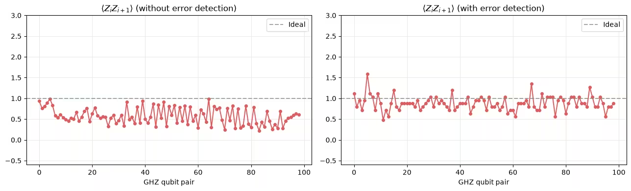
Before detection: <ZiZi+1>=  0.573749999999951
After detection: <ZiZi+1>=  0.8817377312951776

פרשנות התוצאות

שני הגרפים מציגים את $\langle Z_i Z_{i+1}\rangle$ שהוערך מטומוגרפיית shadow עבור כל זוג Qubits שכנים בשרשרת ה-GHZ של 100 Qubits, לפני ואחרי postselection על בדיקות הזוגיות.

עבור מצב GHZ אידיאלי, כל הקורלטורים בין שכנים קרובים שווים ל-$1$. בחומרה, הרעש מוריד את ההערכות הגולמיות ויוצר פיזור בין Qubit ל-Qubit. לאחר זיהוי השגיאות מוסרים snapshots שבהם התרחשה לפחות שגיאה אחת שניתנת לזיהוי, וההערכות הנותרות מתקרבות ל-$1$ עם שונות קטנה יותר, מה שעקבי עם מצב אפקטיבי נקי יותר.

השיפור לאחר זיהוי השגיאות עקבי עם כך שהבדיקות מזהות שגיאות אמיתיות.

השלבים הבאים

כדי ללמוד עוד, עיינו במקורות הבאים:

המלצות

• General formulation of quantum information
• Low-overhead error detection using spacetime codes tutorial
• Qiskit Paulice add-on API documentation

מקורות

• [1] Huang, H. Y., Kueng, R., & Preskill, J. (2020). Predicting many properties of a quantum system from very few measurements. Nature Physics, 16, 1050–1057.

• [2] Zhao, A., Rubin, N. C., & Miyake, A. (2021). Fermionic partial tomography via classical shadows. Phys. Rev. Lett., 127, 110504.

• [3] Low, G. H. (2022). Classical shadows of fermions with particle number symmetry. arXiv:2208.08964.

• [4] Bertoni, C., Haferkamp, J., Hinsche, M. et al. (2024). Shallow Shadows: Expectation Estimation Using Low-Depth Random Clifford Circuits. Phys. Rev. Lett., 133, 020602.

• [5] Hu, H.-Y., Gu, A., Majumder, S. et al. (2025). Demonstration of robust and efficient quantum property learning with shallow shadows. Nature Communications, 16, 2943.

• [6] Martiel, S. & Javadi-Abhari, A. (2025). Low-overhead error detection with spacetime codes. arXiv:2504.15725. © IBM Corp. 2026