התחלת ארגודיות בסקאלות שונות
המחברת הזו מדריכה איך להריץ ולנתח את הניסויים ב-Onset of Ergodicity Across Scales on a Digital Quantum Processor [arXiv:2603.12236]: מהמודל למעגלים, ממחרוזות ביטים לאנטרופיות, מנתונים רועשים לתוצאות מופחתות שגיאות, ומסימולציה של 16 קיוביטים להרצה של 64 קיוביטים על מעבד IBM Quantum® Nighthawk. כל הקוד כאן, וכל פונקציה מוגדרת במקום שבו היא נדרשת לראשונה.
| זמן | סעיף |
|---|---|
| 0–1 דקות | הגדרה |
| 1–6 דקות | 1. מהמודל למעגל |
| 6–12 דקות | 2. מה למדוד ואיך לאמוד זאת |
| 12–19 דקות | 3. רעש, ואיך לבטל אותו |
| 19–24 דקות | 4. הרצה בקנה מידה גדול |
| 24–33 דקות | 5. נתוני החומרה |
| 33–35 דקות | סיכום |
ללכת יחד. הריצו את התאים מלמעלה למטה. אין צורך בחשבון IBM Quantum; התאים שמגישים משימות חומרה כבויים, וסעיף 5 מנתח הרצת חומרה שמורה, שתא ההגדרה מוריד אל data/. שאלות לדיון מסומנות ב-שאלה; נסו לענות לפני שתפתחו את התשובה.
הגדרה
דורש Python 3.12 ומעלה ואת החבילות הבאות:
-
Qiskit SDK גרסה 2.5 ומעלה, עם תמיכה ב-visualization
-
Qiskit Runtime גרסה 0.49 ומעלה (
pip install qiskit-ibm-runtime) -
Qiskit Aer גרסה 0.17 ומעלה (
pip install qiskit-aer) -
Samplomatic גרסה 0.21 ומעלה (
pip install samplomatic) -
NumPy ו-Matplotlib
תא ההגדרה מוריד גם את הרצת החומרה השמורה ואת הייחוסים של MPS (כ-9 MB) אל data/, אלא אם הם כבר שם.
# Added by doQumentation — installs the packages this notebook needs if they are missing
import importlib.util

_needed = {"matplotlib": "matplotlib", "numpy": "numpy", "qiskit": "qiskit", "qiskit_aer": "qiskit-aer", "qiskit_ibm_runtime": "qiskit-ibm-runtime", "samplomatic": "samplomatic"}
_missing = [pip for module, pip in _needed.items()
            if importlib.util.find_spec(module) is None]
# One at a time, so a package that fails to install does not block the others
for _pip in _missing:
    %pip install -q {_pip}
if not _missing:
    print("\u2713 All required packages are installed")
from math import comb
from pathlib import Path
from urllib.request import urlretrieve

import matplotlib.pyplot as plt
import numpy as np
from qiskit import ClassicalRegister, QuantumCircuit, QuantumRegister
from qiskit.primitives import StatevectorSampler
from qiskit.quantum_info import (
    PauliLindbladMap,
    QubitSparsePauli,
    Statevector,
)
from qiskit.transpiler import generate_preset_pass_manager
from qiskit_aer import AerSimulator
from qiskit_aer.noise import NoiseModel, ReadoutError, depolarizing_error
from qiskit_aer.primitives import SamplerV2 as AerSampler

RUN_ON_HARDWARE = (
    False  # True submits the 8x8 jobs in section 4 (needs Nighthawk access)
)
COMPUTE_MPS_REFERENCES = False  # True recomputes the MPS references in section 5 (about 18 minutes)

# Download the saved hardware run and MPS references, unless they are already in data/
data_url = "https://raw.githubusercontent.com/Qiskit/documentation/main/datasets/tutorials/onset-of-ergodicity"
Path("data").mkdir(exist_ok=True)
for name in ("hardware_run.npz", "mps_references_all.npz"):
    if not Path("data", name).exists():
        urlretrieve(f"{data_url}/{name}", Path("data", name))
1. מהמודל למעגל
שער שני הקיוביטים
כל קשר ב-lattice מקבל את אותו שער שני קיוביטים, שמורכב ממסבך (entangler) של הייזנברג ואחריו שדות אקראיים:
כאשר נדגם באופן אחיד מ- עבור כל שער.
שאלה. איך הייתם מפרקים את לשערים שהחומרה יכולה להריץ?
תשובה
השדות קלים. הוא סיבוב חד-קיוביטי על כל קיוביט.
ה-entangler הוא החלק הקשה. , ו- מתחלפים, ולכן הוא מתפרק לשלושה סיבובים, , ו-. כל אחד דורש שני CNOT, מה שנותן שישה CNOT לכל שער.
יש דרך טובה יותר. אפשר לבנות כל שער שני קיוביטים מלכל היותר שלושה CNOT וסיבובים חד-קיוביטיים. המעגל האופטימלי מתחיל מהצורה , ול-entangler הזה כבר יש צורה כזו עם . לכן הוא ממופה ישירות לשלושה CNOT, והזוויות החד-קיוביטיות ליניאריות ב-. קוד הניסוי בונה את השער בדרך הזו.
על חומרה, כל שער שני קיוביטים מוסיף רעש, ולכן חיתוך מספר ה-CNOT בחצי חשוב.
def xxyyzz_gate(circuit, coupling, i, j):
    # exp(iJ(XX + YY + ZZ)) with three CNOTs; only the rotation angles depend on J
    circuit.rz(-np.pi / 2, j)
    circuit.cx(j, i)
    circuit.rz(np.pi / 2 - 2 * coupling, i)
    circuit.ry(2 * coupling - np.pi / 2, j)
    circuit.cx(i, j)
    circuit.ry(np.pi / 2 - 2 * coupling, j)
    circuit.cx(j, i)
    circuit.rz(np.pi / 2, i)

def heisenberg_gate(circuit, coupling, i, j, h_i, h_j):
    # The entangler first, then the random fields exp(i h Z)
    xxyyzz_gate(circuit, coupling, i, j)
    circuit.rz(-2 * h_i, i)
    circuit.rz(-2 * h_j, j)

h_i, h_j = 0.3, -0.7
gate = QuantumCircuit(2)
heisenberg_gate(gate, 0.05 * np.pi, 0, 1, h_i, h_j)
gate.draw("mpl")

ה-brickwork ומחזור Floquet
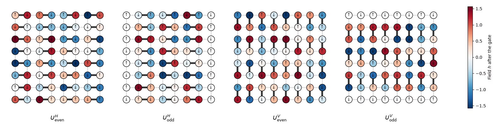
השערים מרצפים את ה-lattice הריבועי בארבע תת-שכבות של קשרים שאינם חופפים, brickwork: קשרים אופקיים שמתחילים בעמודות זוגיות, ואז אי-זוגיות, ואז קשרים אנכיים שמתחילים בשורות זוגיות, ואז אי-זוגיות. הקיוביט נמצא באתר .
def brickwork_layers(num_cols, num_rows):
    # Bonds of the square lattice, in the four sublayers of the brickwork
    def qubit(x, y):
        return y * num_cols + x

    layers = []
    for p in (0, 1):  # horizontal bonds starting on even, then odd, columns
        layers.append(
            [
                (qubit(x, y), qubit(x + 1, y))
                for y in range(num_rows)
                for x in range(p, num_cols - 1, 2)
            ]
        )
    for p in (0, 1):  # vertical bonds starting on even, then odd, rows
        layers.append(
            [
                (qubit(x, y), qubit(x, y + 1))
                for y in range(p, num_rows - 1, 2)
                for x in range(num_cols)
            ]
        )
    return layers

brickwork_layers(4, 4)
[[(0, 1), (2, 3), (4, 5), (6, 7), (8, 9), (10, 11), (12, 13), (14, 15)],
 [(1, 2), (5, 6), (9, 10), (13, 14)],
 [(0, 4), (1, 5), (2, 6), (3, 7), (8, 12), (9, 13), (10, 14), (11, 15)],
 [(4, 8), (5, 9), (6, 10), (7, 11)]]
ארבע תת-השכבות יוצרות מחזור Floquet אחד. המחזור חוזר פעמים עם אותם שדות, כך שהדינמיקה אקראית במרחב ומחזורית בזמן. המעגל מתחיל ממצב Néel, ו- הוא מחצית מאורך הצלע של ה-lattice. התא הבא מצייר מחזור Floquet אחד של ה-lattice בגודל של החומרה, תת-שכבה אחר תת-שכבה, עם השדות של הרצת החומרה, בסגנון איור 5 במאמר. קשרים עבים הם השערים של כל תת-שכבה. כל קיוביט ששער פועל עליו נצבע לפי השדה האקראי שהוא מקבל אחר כך, וקיוביטים בטלים לבנים. החצים מראים את מצב ההתחלה של Néel, כש- מייצג . האיור במאמר מפעיל את התת-שכבות האנכיות קודם; לא צפוי ששום סדר ישנה את הפיזיקה.
# circuit structure, 8x8 system:
side = 8
all_bonds = [bond for layer in brickwork_layers(side, side) for bond in layer]

# get the disorder parameters for a given system:
def sample_disorder(num_cols, num_rows, rng):
    # One pair of fields (h_i, h_j) per gate, reused in every Floquet cycle
    return [
        [
            (bond, tuple(rng.uniform(-np.pi / 2, np.pi / 2, 2)))
            for bond in layer
        ]
        for layer in brickwork_layers(num_cols, num_rows)
    ]

# build the structure for the 8x8 system
example_disorder = sample_disorder(
    side, side, np.random.default_rng(7)
)  # the hardware fields (section 4)
titles = [
    r"$U^H_\mathrm{even}$",
    r"$U^H_\mathrm{odd}$",
    r"$U^V_\mathrm{even}$",
    r"$U^V_\mathrm{odd}$",
]
norm = plt.Normalize(-np.pi / 2, np.pi / 2)
cmap = plt.get_cmap("RdBu_r")

fig, axes = plt.subplots(1, 4, figsize=(16, 4.8), layout="constrained")
for ax, title, sublayer in zip(axes, titles, example_disorder):
    for i, j in all_bonds:
        ax.plot(
            [i % side, j % side],
            [i // side, j // side],
            color="0.75",
            lw=1,
            zorder=0,
        )
    fields = {}
    for (i, j), (h_i, h_j) in sublayer:
        ax.plot(
            [i % side, j % side],
            [i // side, j // side],
            color="0.2",
            lw=4,
            zorder=1,
        )
        fields[i], fields[j] = h_i, h_j
    for q in range(side * side):
        x, y = q % side, q // side
        ax.scatter(
            x,
            y,
            s=260,
            color=cmap(norm(fields[q])) if q in fields else "white",
            edgecolor="black",
            zorder=2,
        )
        ax.text(
            x,
            y,
            "↓" if (x + y) % 2 else "↑",
            ha="center",
            va="center",
            fontsize=9,
            zorder=3,
        )
    ax.set_aspect("equal")
    ax.set_xlim(-1, side)  # padding, so the panels read as separate steps
    ax.set_ylim(side, -1)
    ax.axis("off")
    ax.set_title(title, y=-0.1, fontsize=13)
fig.colorbar(
    plt.cm.ScalarMappable(norm=norm, cmap=cmap),
    ax=axes,
    shrink=0.7,
    label="Field $h$ after the gate",
)
plt.show()
הגדירו את מצב ההתחלה.
# initial state
def neel_state(circuit, num_cols, num_rows, layout):
    for y in range(num_rows):
        for x in range(num_cols):
            if (x + y) % 2 == 1:
                circuit.x(layout[y * num_cols + x])
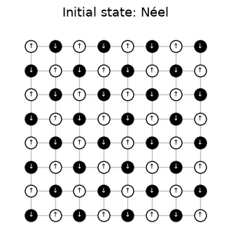
# The initial Néel state: |1⟩ (black, ↓) on odd sites, |0⟩ (white, ↑) on even sites

fig, ax = plt.subplots(figsize=(4, 4.4))
for i, j in all_bonds:
    ax.plot(
        [i % side, j % side],
        [i // side, j // side],
        color="0.75",
        lw=1,
        zorder=0,
    )
for q in range(side * side):
    x, y = q % side, q // side
    excited = (x + y) % 2 == 1
    ax.scatter(
        x,
        y,
        s=150,
        color="black" if excited else "white",
        edgecolor="black",
        zorder=2,
    )
    ax.text(
        x,
        y,
        "↓" if excited else "↑",
        ha="center",
        va="center",
        fontsize=7,
        color="white" if excited else "black",
        zorder=3,
    )
ax.set_aspect("equal")
ax.set_xlim(-1, side)
ax.set_ylim(side, -1)
ax.axis("off")
ax.set_title("Initial state: Néel", fontsize=13)
plt.show()
# actual circuit construction:
def heisenberg_floquet_circuit(
    num_cols, num_rows, coupling, num_cycles, disorder, measure=True
):
    num_qubits = num_cols * num_rows
    circuit = QuantumCircuit(num_qubits)
    neel_state(circuit, num_cols, num_rows, list(range(num_qubits)))
    cycle = QuantumCircuit(num_qubits)
    for sublayer in disorder:
        for (i, j), (h_i, h_j) in sublayer:
            heisenberg_gate(cycle, coupling, i, j, h_i, h_j)
    for _ in range(num_cycles):
        circuit.compose(cycle, inplace=True)
    if measure:
        circuit.measure_all()
    return circuit
דוגמה של
הסימולציות משתמשות ב-lattice של עם שני מחזורים, ובצימודים שנחקרו במאמר. קבוצה אחת של שדות משמשת שוב לכל צימוד.
# simulation parameters:
num_cols = num_rows = 4
num_qubits = num_cols * num_rows
num_cycles = 2
couplings = (
    np.array([0.005, 0.01, 0.02, 0.03, 0.04, 0.05, 0.06, 0.08, 0.10, 0.125])
    * np.pi
)
disorder = sample_disorder(num_cols, num_rows, np.random.default_rng(42))

# circuit construction:
logical_circuits = [
    heisenberg_floquet_circuit(
        num_cols, num_rows, coupling, num_cycles, disorder
    )
    for coupling in couplings
]
logical_circuits[5].draw(output="mpl", fold=-1)

# transpiling the circuit:
pass_manager = generate_preset_pass_manager(
    optimization_level=3,
    basis_gates=["cz", "rz", "sx", "x"],
    seed_transpiler=7,
)
circuits = [pass_manager.run(circuit) for circuit in logical_circuits]

def two_qubit_stats(circuit):
    count = sum(1 for inst in circuit.data if inst.operation.num_qubits == 2)
    depth = circuit.depth(lambda inst: inst.operation.num_qubits == 2)
    return count, depth

stats = {two_qubit_stats(circuit) for circuit in circuits}
assert len(stats) == 1, "the CZ structure should not depend on J"
num_cz, depth = stats.pop()
print(
    f"{num_qubits} qubits: {num_cz} CZ gates in {depth} layers, for every coupling"
)
circuits[5].draw("mpl", fold=-1, scale=0.4)
16 qubits: 144 CZ gates in 24 layers, for every coupling

אין צורך במהדר חכם, כי המעגלים (והניסוי) תוכננו עבור IBM Nighthawk.
סימולציה של ה-lattice בגודל
עבור ה-lattice בגודל , אפשר לעשות את שני הדברים: לחשב את המצב המדויק בכל צימוד, ולדגום כל מעגל עם 10,000 shots, כמו בניסוי. ה-shots נשמרים בצורה (אצוות, shots, קיוביטים), באותה פריסה כמו ה-randomizations בנתוני החומרה. כאן כל 10,000 ה-shots יוצרים אצווה אחת, ולכן ה-bootstrap על פני אצוות לא מוסיף רעש shots, ופסי השגיאה בגרף הבא מציגים רק את הפיזור בין מיקומי ה-marginal.
exact_states = [
    Statevector(
        heisenberg_floquet_circuit(
            num_cols, num_rows, c, num_cycles, disorder, measure=False
        )
    )
    for c in couplings
]

shots = 10_000
results = (
    StatevectorSampler(default_shots=shots, seed=1234).run(circuits).result()
)

# the output of the simulation for the 10 couplings
bits = [
    result.data.meas.to_bool_array(order="little").reshape(
        1, 10_000, num_qubits
    )
    for result in results
]

print(bits[0])
[[[False  True False ... False  True False]
  [False  True False ... False  True False]
  [False  True False ... False  True False]
  ...
  [False  True False ... False  True False]
  [False  True False ... False  True False]
  [False  True False ... False  True False]]]
2. מה למדוד ואיך לאמוד זאת
ה-IPR ואנטרופיית ההתנגשות
עבור marginal של קיוביטים עם התפלגות מחרוזות ביטים , הגודל שיש לאמוד הוא inverse participation ratio (IPR) של ההתפלגות השולית, ומתוכו אנטרופיית ההתנגשות:
הוא גם ההסתברות ששני shots מסכימים על ה-marginal. למצב מכפלה יש , ולמצב אקראי יש , ולכן עולה מ-0 לכ- ביטים ככל שה-marginal נעשה אקראי.
אומדן 1: ספירת זוגות של shots
שאלה. איך אומדים את הגודל הזה מה-shots שלכם?
תשובה
האומדן הנאיבי מחשב כל מה-shots בתור , ואז מסכם . האומדן הזה מוטה.
סופר כל shot כמסכים עם עצמו, מה שמעלה את האומדן: בממוצע הוא נותן במקום . מכיוון ש- היא ההסתברות ששני shots מסכימים, סופרים רק זוגות של shots שונים:
האומדן הזה בלתי מוטה, וזה מה ש-ipr_from_shots שלהלן מחשב.
# IPR expectation values:

# refactor this function cause it does not scale
def ipr_from_shots(bits):
    # Pair-counting estimate of the IPR of a marginal: the fraction of pairs of different shots
    # that agree on it. bits holds the marginal's qubits only, with shape (randomizations, shots,
    # qubits), and all randomizations are pooled.
    n = bits.shape[-1]
    outcomes = bits @ 2 ** np.arange(
        n
    )  # each shot's marginal bitstring, read as an integer
    counts = np.bincount(outcomes.ravel())  # how often each outcome occurs
    total = counts.sum()
    return float((counts * (counts - 1)).sum() / (total * (total - 1)))

def collision_entropy(ipr):
    return -np.log2(ipr)
אומדן 2: פיתוח Parseval
אפשר לכתוב את ה-IPR גם דרך הפריטיות של כל תת-הקבוצות הלא ריקות של ה-marginal:
הצורה הזו חשובה כי שיטות להפחתת שגיאות כמו PEA עובדות על ערכי תצפית, לא על הסתברויות. קיוביט אחד: הסתברויות התוצאה הן ו-, ולכן
שולי : כשה-qubits שלו מסומנים , לשוליים יש זוגיויות: 4 qubits בודדים, 6 זוגות, 4 שלשות, והשוליים כולם, ולכן
def parity_supports(patch):
    # All nonempty subsets S of the marginal
    return sorted(
        [
            tuple(q for k, q in enumerate(patch) if mask & (1 << k))
            for mask in range(1, 1 << len(patch))
        ],
        key=len,
    )

def parity_expectation_values(bits, supports):
    # Shot-averaged <Z_S> for every support, per randomization
    signs = 1 - 2 * bits.astype(np.int8)
    return np.stack(
        [signs[..., list(s)].prod(axis=-1).mean(axis=-1) for s in supports],
        axis=-1,
    )

# Example: the parities of a 3-qubit marginal made of lattice qubits 5, 6, and 9
print(parity_supports([5, 6, 9]))
print(f"A 3×3 marginal has {len(parity_supports(range(9)))} parities")
[(5,), (6,), (9,), (5, 6), (5, 9), (6, 9), (5, 6, 9)]
A 3×3 marginal has 511 parities
ממוצע על פני שוליים
פונקציות שימושיות נוספות: ערכי Haar, בחירת שוליים, bootstrapping וחישוב ממוצעים.
# functions for the Haar values on plots:
def haar_ipr(num_patch, num_qubits):
    # Mean IPR of a marginal for Haar-random states in the sector with num_qubits // 2 ones
    weight = num_qubits // 2
    dimension = comb(num_qubits, weight)
    total = 0
    for k in range(num_patch + 1):  # k ones on the marginal
        rest = (
            comb(num_qubits - num_patch, weight - k) if weight - k >= 0 else 0
        )
        total += comb(num_patch, k) * rest * (rest + 1)
    return total / (dimension * (dimension + 1))

def haar_entropy(num_patch, num_qubits):
    return collision_entropy(haar_ipr(num_patch, num_qubits))

# definitions of positions in the lattice:
def patch_qubits(anchor, shape, num_cols):
    # Lattice indices of a rectangular marginal with its top-left corner at anchor
    (x0, y0), (width, height) = anchor, shape
    return [
        (y0 + dy) * num_cols + (x0 + dx)
        for dy in range(height)
        for dx in range(width)
    ]

def all_positions(shape, num_cols, num_rows):
    # Every placement of a (width, height) marginal on the lattice
    width, height = shape
    return [
        patch_qubits((x, y), shape, num_cols)
        for y in range(num_rows - height + 1)
        for x in range(num_cols - width + 1)
    ]

# bootstrapping for error bars:
bootstrap_rng = np.random.default_rng(0)

def bootstrap_error(statistic, *samples, axis=0, num_resamples=50):
    # Shot noise of a statistic, from resampling the randomizations (along axis of every
    # sample) with replacement
    values = []
    for _ in range(num_resamples):
        resampled = [
            np.take(
                x,
                bootstrap_rng.integers(0, x.shape[axis], x.shape[axis]),
                axis=axis,
            )
            for x in samples
        ]
        values.append(statistic(*resampled))
    return float(np.std(values, ddof=1))

# averaging the ipr over marginals:
def average_ipr(iprs, shot_errors):
    # iprs and shot_errors have shape (positions, couplings). The mean IPR over positions, and its
    # error: the spread between positions plus the shot noise of each (law of total variance)
    iprs, shot_errors = np.asarray(iprs), np.asarray(shot_errors)
    count = len(iprs)
    variance = (
        iprs.var(axis=0, ddof=1) / count
        + (shot_errors**2).sum(axis=0) / count**2
    )
    return iprs.mean(axis=0), np.sqrt(variance)
# Calculating exact simulation entropies:
patch_shapes = {
    "1×1": (1, 1),
    "1×2": (2, 1),
    "2×2": (2, 2),
    "2×3": (3, 2),
    "3×3": (3, 3),
}

# calculate the exact entropies:
sim_positions = {
    label: all_positions(shape, num_cols, num_rows)
    for label, shape in patch_shapes.items()
}
exact_iprs = {  # shape (positions, couplings)
    label: np.array(
        [
            [(s.probabilities(qargs=q) ** 2).sum() for s in exact_states]
            for q in qubit_lists
        ]
    )
    for label, qubit_lists in sim_positions.items()
}
exact_entropies = {
    label: collision_entropy(v.mean(axis=0))
    for label, v in exact_iprs.items()
}

# Average IPR of every shape over its positions, from the sampled shots, then the entropy
iprs_from_shots = {}  # per shape: average IPR and its error, at every coupling
entropies_from_shots = {}  # per shape: average entropy and its error, at every coupling
for label, qubit_lists in sim_positions.items():
    iprs = [[ipr_from_shots(b[:, :, q]) for b in bits] for q in qubit_lists]

    # bootstrapping over subsampling for error bars:
    errors = [
        [bootstrap_error(ipr_from_shots, b[:, :, q]) for b in bits]
        for q in qubit_lists
    ]
    ipr, ipr_error = average_ipr(iprs, errors)
    iprs_from_shots[label] = (ipr, ipr_error)
    entropies_from_shots[label] = (
        collision_entropy(ipr),
        ipr_error / (ipr * np.log(2)),
    )
# Now plot the average IPR on the left, and the same averages as entropies on the right
colors = plt.cm.plasma(np.linspace(0.05, 0.8, len(patch_shapes)))
fig, (ax_ipr, ax_entropy) = plt.subplots(1, 2, figsize=(12.8, 4.2))
for (label, qubit_lists), color in zip(sim_positions.items(), colors):
    n = len(qubit_lists[0])
    ipr, ipr_error = iprs_from_shots[label]
    entropy, entropy_error = entropies_from_shots[label]
    # Left: the average IPR, with its exact value and its random-state value
    ax_ipr.axhline(haar_ipr(n, num_qubits), color=color, ls="dashdot", lw=0.9)
    ax_ipr.plot(
        couplings / np.pi, exact_iprs[label].mean(axis=0), color=color
    )
    ax_ipr.errorbar(
        couplings / np.pi,
        ipr,
        yerr=ipr_error,
        fmt="o",
        color=color,
        mec="white",
        ms=7,
        capsize=3,
        label=f"{label} ({len(qubit_lists)} positions)",
    )
    # Right: the average collision entropy
    ax_entropy.axhline(
        haar_entropy(n, num_qubits), color=color, ls="dashdot", lw=0.9
    )
    ax_entropy.plot(couplings / np.pi, exact_entropies[label], color=color)
    ax_entropy.errorbar(
        couplings / np.pi,
        entropy,
        yerr=entropy_error,
        fmt="o",
        color=color,
        mec="white",
        ms=7,
        capsize=3,
        label=f"{label} ({len(qubit_lists)} positions)",
    )
ax_ipr.set_yscale("log")
ax_ipr.set_ylabel("Average IPR")
ax_entropy.set_ylabel("Average collision entropy (bits)")
for ax in (ax_ipr, ax_entropy):
    ax.set_xlabel("Coupling $J/\\pi$")
fig.suptitle("Exact (lines) and sampled (dots), 4×4 lattice, 2 cycles")
ax_entropy.legend(title="Marginal", loc="upper left")
fig.tight_layout()
plt.show()
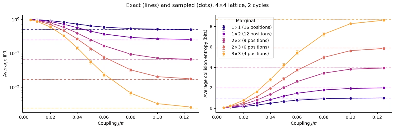
צורת השוליים כולן עולות בהדרגה לעבר הערך של מצב אקראי, ושוליים גדולים יותר מגיעים אליו ב- גדול יותר.
3. רעש, ואיך מבטלים אותו
סימולציה רועשת
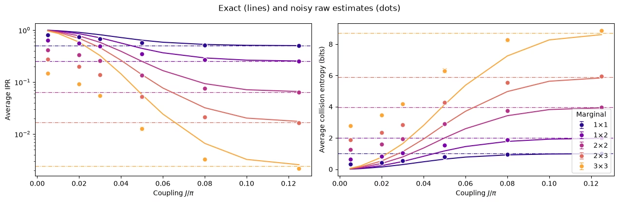
עכשיו נוסיף רעש: רעש דה-פולריזציה של 1% על שני qubits בכל שער CZ ושגיאת קריאה של 3% בכל qubit, כשהדגימה נעשית עם ה-Sampler של Qiskit Aer. עם 144 שערי CZ במעגל, זה הרבה פחות רעש ממה שמעגלי החומרה בגודל 8×8 חווים, אבל מספיק כדי לראות את השפעתו. הסימולציה משתמשת בשישה צימודים וב-4,000 shots לכל אחד, והיא נמשכת כדקה וחצי.
שאלה. לפני שתריצו: האם הרעש יגרום למערכת להיראות תרמלית יותר או פחות?
תשובה
יותר. הרעש מערבב את התוצאות, מה שמקרב כל התפלגות שוליים להתפלגות אחידה, ולכן ה-IPR הגולמי יורד והאנטרופיה עולה. בלי mitigation, הרעש נראה כמו תרמליזציה שאינה קיימת, והמעברים מתרחשים מוקדם מדי.
# define the noise model

noise_model = NoiseModel()
# two qubit depolarizing noise:
noise_model.add_all_qubit_quantum_error(depolarizing_error(0.01, 2), ["cz"])
# symmetric readout noise:
noise_model.add_all_qubit_readout_error(
    ReadoutError([[0.97, 0.03], [0.03, 0.97]])
)

# simulation is done using trajectories
noisy_sampler = AerSampler(
    default_shots=4000,
    seed=1,
    options={"backend_options": {"noise_model": noise_model}},
)

# choose a subset of J values for speed:
noisy_indices = [
    0,
    2,
    3,
    5,
    7,
    9,
]  # J/π = 0.005, 0.02, 0.03, 0.05, 0.08, 0.125
noisy_results = noisy_sampler.run(
    [circuits[k] for k in noisy_indices]
).result()

# No twirling here, so the 20 "randomizations" are just batches of 200 shots
noisy_bits = {
    k: result.data.meas.to_bool_array(order="little").reshape(
        20, 200, num_qubits
    )
    for k, result in zip(noisy_indices, noisy_results)
}
# Calculating noisy entropies

# Average IPR of every shape over its positions, from the noisy shots, then the entropy
noisy_iprs = {}  # per shape: average IPR and its error, at every noisy coupling
noisy_entropies = {}  # per shape: average entropy and its error, at every noisy coupling
for label, qubit_lists in sim_positions.items():
    iprs = [
        [ipr_from_shots(noisy_bits[k][:, :, q]) for k in noisy_indices]
        for q in qubit_lists
    ]

    # bootstrapping over subsampling for error bars:
    errors = [
        [
            bootstrap_error(ipr_from_shots, noisy_bits[k][:, :, q])
            for k in noisy_indices
        ]
        for q in qubit_lists
    ]
    ipr, ipr_error = average_ipr(iprs, errors)
    noisy_iprs[label] = (ipr, ipr_error)
    noisy_entropies[label] = (
        collision_entropy(ipr),
        ipr_error / (ipr * np.log(2)),
    )
fig, (ax_ipr, ax_entropy) = plt.subplots(1, 2, figsize=(12.8, 4.2))
for (label, qubit_lists), color in zip(sim_positions.items(), colors):
    n = len(qubit_lists[0])
    ipr, ipr_error = noisy_iprs[label]
    entropy, entropy_error = noisy_entropies[label]
    # Left: the average IPR, with its exact value and its random-state value
    ax_ipr.axhline(haar_ipr(n, num_qubits), color=color, ls="dashdot", lw=0.9)
    ax_ipr.plot(
        couplings / np.pi, exact_iprs[label].mean(axis=0), color=color
    )
    ax_ipr.errorbar(
        couplings[noisy_indices] / np.pi,
        ipr,
        yerr=ipr_error,
        fmt="o",
        color=color,
        mec="white",
        ms=7,
        capsize=3,
        label=label,
    )
    # Right: the same averages as entropies
    ax_entropy.axhline(
        haar_entropy(n, num_qubits), color=color, ls="dashdot", lw=0.9
    )
    ax_entropy.plot(couplings / np.pi, exact_entropies[label], color=color)
    ax_entropy.errorbar(
        couplings[noisy_indices] / np.pi,
        entropy,
        yerr=entropy_error,
        fmt="o",
        color=color,
        mec="white",
        ms=7,
        capsize=3,
        label=label,
    )
ax_ipr.set_yscale("log")
ax_ipr.set_ylabel("Average IPR")
ax_entropy.set_ylabel("Average collision entropy (bits)")
for ax in (ax_ipr, ax_entropy):
    ax.set_xlabel("Coupling $J/\\pi$")
fig.suptitle("Exact (lines) and noisy raw estimates (dots)")
ax_entropy.legend(title="Marginal", loc="lower right")
fig.tight_layout()
plt.show()
סיעור מוחות: איך הייתם מבטלים את זה?
גישה מוצעת
ב- קטן, המצב כמעט אינו שזור, ולכן התשובה האידיאלית שם זולה לחישוב קלאסי, אפילו עבור 64 qubits. זה מרמז שאפשר למדוד את השפעת הרעש בצימוד כיול קטן ולתקן בעזרתה כל צימוד אחר. יש שתי דרכים טבעיות לעשות זאת, הנקראות כיול בשזירה נמוכה (LEC):
LEC על ה-IPR. משנים את קנה המידה של העודף של ה-IPR מעל ערכו עבור התפלגות אחידה, , בגורם אחד לכל שוליים:
LEC על ערכי התצפית של . משנים את קנה המידה של כל זוגיות בשוליים בגורם משלה, ובונים מחדש את ה-IPR בעזרת נוסחת Parseval:
בקוד, מכל זוגיות מוגדלת בריבוע מחסירים את השונות שלה כדי להסיר הטיה, כמו בסעיף 2.
שתי השיטות זהות אם כל שווה ל-.
Question. What are the pros and cons of these methods?
תשובה
Pros
-
זול: לא נדרשים נתונים נוספים מההתקן, רק סימולציה קלאסית ב-.
-
מנצל את מבנה המעגל: עומק המעגל ושכבות ה-CZ אינם משתנים עם , ולכן הרעש ב- הוא אותו רעש כמו בכל אחר.
Cons
- מניח שהשפעת הרעש על הגדלים הנמדדים אינה תלויה ב-: הרעש עצמו זהה, אבל האופן שבו הוא מדכא את ה-IPR או כל יכול להשתנות ככל ש- גדל.
שתי השיטות על הסימולציה הרועשת
# function to mitigate the IPR signal:
def mitigate_ipr_w_lec(
    ipr_raw, ipr_raw_calibration, ipr_ideal_calibration, num_patch
):
    # LEC on the IPR: one factor R0 for the excess over the uniform value
    uniform = 2.0**-num_patch
    factor = (ipr_ideal_calibration - uniform) / (
        ipr_raw_calibration - uniform
    )
    return uniform + factor * (ipr_raw - uniform)

# function used to calculate the target <Z> expectation values
def parities_from_probabilities(probabilities):
    # Ideal <Z_S> from a marginal distribution, in parity_supports order: subsets
    # by size, and in bitmask order within each size
    outcomes = np.arange(len(probabilities))
    masks = np.array(sorted(range(1, len(probabilities)), key=int.bit_count))
    signs = (-1.0) ** np.bitwise_count(outcomes[:, None] & masks[None, :])
    return np.asarray(probabilities) @ signs

# calculate boosting factors:
def lec_z_factors(calibration_parities, ideal_parities):
    # LEC on <Z>: one factor r_S per parity, from data with shape (randomizations, supports).
    return ideal_parities / calibration_parities.mean(axis=0)

# function to mitigate the IPR from <Z> expectation values:
def mitigate_ipr_w_lec_on_parities(
    parities, calibration_parities, ideal_calibration_parities, num_patch
):
    # LEC on <Z>: rescale each parity by its factor r_S = ideal / raw at J0, then rebuild the IPR
    # with Parseval. parities and calibration_parities have shape (randomizations, supports).
    # Each squared, rescaled parity is debiased by subtracting its variance, which to first
    # order combines the shot noise at J. The shot noise of r_S from J0 is omitted; including it
    # does not change the results.
    factors = lec_z_factors(calibration_parities, ideal_calibration_parities)
    mean = parities.mean(axis=0)  # mean over the twirling instances
    variance = parities.var(axis=0, ddof=1) / len(
        parities
    )  # variance of the mean
    rescaled = factors * mean
    rescaled_variance = factors**2 * variance
    return float((1 + np.sum(rescaled**2 - rescaled_variance)) / 2**num_patch)
def lec_estimates(patch_bits, parities, ideal, calibration, num_patch):
    # LEC on the IPR and on <Z> for one marginal position, at every coupling: values and shot
    # noise. patch_bits (the bits of the marginal only) and parities are per coupling, with
    # randomizations first.
    q_ideal = (ideal**2).sum()
    ideal_parities = parities_from_probabilities(ideal)

    def ipr_statistic(b, c):
        return mitigate_ipr_w_lec(
            ipr_from_shots(b), ipr_from_shots(c), q_ideal, num_patch
        )

    def z_statistic(p, c):
        return mitigate_ipr_w_lec_on_parities(p, c, ideal_parities, num_patch)

    values = {"LEC on IPR": [], "LEC on ⟨Z⟩": []}
    errors = {"LEC on IPR": [], "LEC on ⟨Z⟩": []}
    for k in range(len(patch_bits)):
        if (
            k == calibration
        ):  # both match the ideal value at J0 by construction
            for method in values:
                values[method].append(q_ideal)
                errors[method].append(0.0)
            continue
        values["LEC on IPR"].append(
            ipr_statistic(patch_bits[k], patch_bits[calibration])
        )
        errors["LEC on IPR"].append(
            bootstrap_error(
                ipr_statistic, patch_bits[k], patch_bits[calibration]
            )
        )
        values["LEC on ⟨Z⟩"].append(
            z_statistic(parities[k], parities[calibration])
        )
        errors["LEC on ⟨Z⟩"].append(
            bootstrap_error(z_statistic, parities[k], parities[calibration])
        )
    return values, errors

# getting all the data:
calibration_index = 0  # index of J0 = 0.005π in noisy_indices
mitigated = {
    "LEC on IPR": {},
    "LEC on ⟨Z⟩": {},
}  # per shape: (values, errors), each (positions, couplings)
for label, qubit_lists in sim_positions.items():
    n = len(qubit_lists[0])
    per_position = []
    for qubits in qubit_lists:
        supports = parity_supports(qubits)
        parities = [
            parity_expectation_values(noisy_bits[k], supports)
            for k in noisy_indices
        ]
        patch_bits = [noisy_bits[k][:, :, qubits] for k in noisy_indices]
        ideal = exact_states[noisy_indices[calibration_index]].probabilities(
            qargs=qubits
        )
        per_position.append(
            lec_estimates(patch_bits, parities, ideal, calibration_index, n)
        )
    for method in mitigated:
        mitigated[method][label] = (
            [p[0][method] for p in per_position],
            [p[1][method] for p in per_position],
        )

# Average over positions, then the entropy, for both methods
mitigated_entropies = {
    method: {} for method in mitigated
}  # per method and shape: entropy and its error
for method, by_shape in mitigated.items():
    for label, (values, errors) in by_shape.items():
        ipr, ipr_error = average_ipr(values, errors)
        mitigated_entropies[method][label] = (
            collision_entropy(ipr),
            ipr_error / (ipr * np.log(2)),
        )  # log here comes from error propagation
# Plot the data mitigated with both methods:

fig, axes = plt.subplots(1, 2, figsize=(12.8, 4.2), sharey=True)
for ax, (method, by_shape) in zip(axes, mitigated_entropies.items()):
    for (label, qubit_lists), color in zip(sim_positions.items(), colors):
        entropy, error = by_shape[label]
        ax.axhline(
            haar_entropy(len(qubit_lists[0]), num_qubits),
            color=color,
            ls="dashdot",
            lw=0.9,
        )
        ax.plot(couplings / np.pi, exact_entropies[label], color=color)
        ax.errorbar(
            couplings[noisy_indices] / np.pi,
            entropy,
            yerr=error,
            fmt="o",
            color=color,
            mec="white",
            ms=7,
            capsize=3,
            label=label,
        )
    ax.set_title(f"{method} (lines: exact)")
    ax.set_xlabel("Coupling $J/\\pi$")
axes[0].set_ylabel("Average collision entropy (bits)")
axes[0].legend(title="Marginal", loc="lower right")
fig.tight_layout()
plt.show()

# add the noisy data here too
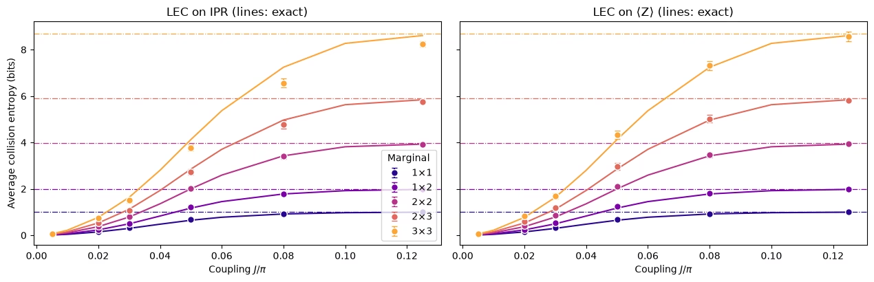
שתי השיטות מסירות את רוב הנזק: האומדנים הגולמיים בגרף הקודם אקראיים מדי, והמתוקנים עוקבים אחרי העקומות המדויקות. ההבדלים מתגלים בשוליים הגדולים יותר.
בשוליים הקטנים שתי השיטות עובדות. עבור שוליים , LEC על קרובה בבירור יותר.
למה LEC על ה-IPR נותנת אנטרופיה נמוכה מדי. אנטרופיה נמוכה מדי פירושה שה-IPR גדול מדי: LEC על ה-IPR מנפחת אותו יתר על המידה. היא מניחה שהרעש מדכא את התרומה של כל ל-IPR באותו גורם. ב-, כל קרוב ל-, ולכן כל המחרוזות תורמות באופן שווה, ורוב המחרוזות הן במשקל בינוני: מתוך 511 המחרוזות של שוליים , ל-252 יש משקל 4 או 5, ורק לתשע יש משקל 1. הרעש מדכא מחרוזת יותר ככל שמשקלה גבוה יותר (שגיאת הקריאה לבדה מדכאת מחרוזת במשקל ב-), ולכן הגורם היחיד נקבע בעיקר לפי דיכוי של מחרוזות במשקל בינוני. ככל ש- גדל, ה- במשקל הגבוה ביותר דועכים מהר ביותר, וה-IPR נשען יותר ויותר על מחרוזות במשקל נמוך, שהרעש מדכא פחות. הגדלה שלהן בגורם שנלמד בעיקר ממחרוזות מדוכאות יותר מנפחת את ה-IPR יתר על המידה. ההשפעה גדלה עם גודל השוליים, כי לשוליים גדולים יותר יש טווח משקלים רחב יותר. היא הגדולה ביותר ב- בינוני, אחרי שהתמהיל של המחרוזות השתנה אך בזמן שהעודף של ה-IPR מעל ערכו האחיד עדיין משמעותי.
למה LEC על טועה לכיוון ההפוך. היא משנה את קנה המידה של כל מחרוזת בגורם משלה, ולכן המעבר בין משקלים אינו משפיע עליה. היא מניחה רק שכל מחרוזת שומרת על הדיכוי שלה ב-. ככל ש- גדל, כל מתפשט לאופרטורים במשקל גבוה יותר, שקולטים יותר רעש מאשר ב-, ולכן הגורמים מתקנים מעט פחות מדי והאנטרופיה יוצאת מעט גבוהה מדי.
לכן התחזית לבדיקה בחומרה היא: ככל ששוליים גדולים יותר, כך LEC על אמורה לנצח יותר. בחומרה, הרעש חזק יותר ואינו בצורה ידועה.
4. הרצה בקנה מידה גדול
ניסוי החומרה מריץ סריג עם ארבעה מחזורים: 64 qubits ו-1,344 שערי CZ ב-48 שכבות, בתשעה צימודים. חמישה דברים משתנים בהשוואה לסימולציה:
-
את הרעש צריך ללמוד, וזה עובד רק אם שכבות ה-CZ קבועות.
-
Twirling הופך את הרעש של כל שכבה לערוץ Pauli, שאפשר ללמוד ולהגביר.
-
Dynamical decoupling (DD) מגן על qubits בטלים.
-
הגברת רעש עבור PEA רצה באותו job עם הנתונים הראשיים.
-
סימולציות MPS ב- קטן מספקות את ההפניות הקלאסיות עבור mitigation שגיאות מבוסס LEC.
התאים שזקוקים ל-backend רצים רק כאשר RUN_ON_HARDWARE הוא True. אפשר להריץ מחדש סימולציות MPS כאשר COMPUTE_MPS_REFERENCES מוגדר ל-True. שאר התאים רצים כאן.
# hardware run parameters:
num_cols_hw = num_rows_hw = 8
num_qubits_hw = num_cols_hw * num_rows_hw
num_cycles_hw = 4
couplings_hw = (
    np.array([0.005, 0.01, 0.02, 0.03, 0.05, 0.07, 0.09, 0.11, 0.125]) * np.pi
)
calibration_hw = 0  # J0 = 0.005π
disorder_hw = sample_disorder(
    num_cols_hw, num_rows_hw, np.random.default_rng(7)
)

# if running PEA:
noise_factors = np.array([1.0, 1.5, 2.0])  # PEA noise-amplification factors
שכבות CZ קבועות
def compile_by_sublayer(
    num_cols,
    num_rows,
    coupling,
    num_cycles,
    disorder,
    pass_manager,
    layout=None,
    num_physical_qubits=None,
):
    # Compile each sublayer once and repeat it with barriers, so the CZ layers are the
    # same in every cycle and at every coupling. The registers are named explicitly
    # because register names enter Samplomatic's box hashes. Bits land in lattice order.
    num_qubits = num_cols * num_rows
    if layout is None:
        layout, num_physical_qubits = list(range(num_qubits)), num_qubits
    blocks = []
    for sublayer in disorder:
        block = QuantumCircuit(num_qubits)
        for (i, j), (h_i, h_j) in sublayer:
            heisenberg_gate(block, coupling, i, j, h_i, h_j)
        blocks.append(pass_manager.run(block))
    circuit = QuantumCircuit(
        QuantumRegister(num_physical_qubits, "q"),
        ClassicalRegister(num_qubits, "meas"),
    )
    neel_state(circuit, num_cols, num_rows, layout)
    for _ in range(num_cycles):
        for block in blocks:
            circuit.compose(block, inplace=True)
            circuit.barrier(layout)
    circuit.measure(layout, range(num_qubits))
    return circuit
קופסאות ללימוד רעש
לאחר מכן מנהל המעברים (pass manager) של Samplomatic מקבץ כל מעגל ל-קופסאות: אחת לכל שכבת CZ ואחת למדידות. כל קופסה נושאת הפניה למודל הרעש שהיא צריכה, כך שאפשר לבדוק שכל הצימודים חולקים את אותן קופסאות. התא הבא עושה זאת עבור מעגלי של הרצת החומרה, מקומפלים לשערי CZ בלי backend, ומדפיס את הקופסאות שלימוד הרעש יאפיין.
from samplomatic import build
from samplomatic.transpiler import generate_boxing_pass_manager
from samplomatic.utils import find_unique_box_instructions

boxing_pass_manager = generate_boxing_pass_manager(
    enable_gates=True,  # twirl the CZ layers
    enable_measures=True,  # twirl the measurements
    inject_noise_targets="gates",  # PEA amplifies the noise of the CZ layers only
    inject_noise_strategy="uniform_modification",
)

def noise_refs(boxed_circuit):
    return sorted(
        annotation.ref
        for box in find_unique_box_instructions(boxed_circuit.data)
        for annotation in box.operation.annotations
        if hasattr(annotation, "ref")
    )

# The 8x8 hardware circuits, compiled to CZ gates on the lattice qubits (no backend needed)
compiled_8x8 = [
    compile_by_sublayer(
        num_cols_hw, num_rows_hw, c, num_cycles_hw, disorder_hw, pass_manager
    )
    for c in couplings_hw
]
boxed_8x8 = [boxing_pass_manager.run(circuit) for circuit in compiled_8x8]
assert all(
    noise_refs(b) == noise_refs(boxed_8x8[0]) for b in boxed_8x8
), "layers differ between couplings"
num_cz, depth = two_qubit_stats(compiled_8x8[0])
print(
    f"{num_qubits_hw} qubits: {num_cz} CZ gates in {depth} layers, for every coupling"
)
for box in find_unique_box_instructions(boxed_8x8[0].data):
    ops = box.operation.blocks[0].count_ops()
    print(
        f"{box.operation.num_qubits}-qubit box: {ops.get('cz', 0)} CZ, {ops.get('measure', 0)} measurements"
    )
print(
    f"All {len(boxed_8x8)} couplings share these {len(find_unique_box_instructions(boxed_8x8[0].data))} boxes"
)
64 qubits: 1344 CZ gates in 48 layers, for every coupling
64-qubit box: 32 CZ, 0 measurements
64-qubit box: 24 CZ, 0 measurements
64-qubit box: 32 CZ, 0 measurements
64-qubit box: 24 CZ, 0 measurements
64-qubit box: 0 CZ, 64 measurements
All 9 couplings share these 5 boxes
Twirl של המעגלים
בכל אקראיזציה, Samplomatic מוסיף שערי Pauli אקראיים לפני כל קופסה ושערים מפצים אחריה, ממוזגים לתוך שערי ה-qubit הבודד השכנים. בממוצע על פני אקראיזציות, הרעש של כל שכבה הופך לערוץ Pauli, ש-NoiseLearnerV3 יכול ללמוד כמודל Pauli-Lindblad דליל ושלב PEA יכול להגביר. Twirling של המדידה הופך ביטים באקראי לפני הקריאה. ההיפוכים מבוטלים בתוכנה, מה שהופך את רעש הקריאה לסימטרי והוא הבסיס לתיקון הקריאה (TREX).
תהליך העבודה בחומרה
בוחרים את ה-qubits, מקמפלים את המעגלים, ואז לומדים את הרעש ומריצים את הסריקה. התאים האלה כבויים כאן.
בחירת ה-qubits. הרשת הריבועית של Nighthawk מכילה את סריג בלי שערי SWAP. התא מדרג כל מלבן ברשת לפי שגיאות ה-CZ והקריאה המדווחות שלו ובוחר את הטוב ביותר.
def square_layouts(backend, side):
    # Every side x side rectangle of the square qubit grid that supports all bonds
    target = backend.target

    def has_cz(a, b):
        return (a, b) in target["cz"] or (b, a) in target["cz"]

    stride = next(
        s
        for s in (10, 12)
        if all(has_cz(q, q + s) for q in range(backend.num_qubits - s))
    )
    layouts = []
    for y0 in range(backend.num_qubits // stride - side + 1):
        for x0 in range(stride - side + 1):
            layout = [
                stride * (y0 + y) + x0 + x
                for y in range(side)
                for x in range(side)
            ]
            bonds = [
                bond
                for layer in brickwork_layers(side, side)
                for bond in layer
            ]
            if all(has_cz(layout[i], layout[j]) for i, j in bonds):
                layouts.append(((x0, y0), layout))
    return layouts

def layout_score(backend, layout, side, uses_per_bond):
    # Minus the summed log-fidelity of the bonds (each used uses_per_bond times) and readouts
    properties, target = backend.properties(), backend.target
    cz_errors = []
    for i, j in (
        bond for layer in brickwork_layers(side, side) for bond in layer
    ):
        pair = (
            (layout[i], layout[j])
            if (layout[i], layout[j]) in target["cz"]
            else (layout[j], layout[i])
        )
        cz_errors.append(properties.gate_error("cz", pair))
    readout_errors = [properties.readout_error(q) for q in layout]
    if max(cz_errors) >= 0.5 or max(readout_errors) >= 0.25:
        return np.inf  # an unusable qubit or bond
    return float(
        -uses_per_bond * np.log1p(-np.array(cz_errors)).sum()
        - np.log1p(-np.array(readout_errors)).sum()
    )

if RUN_ON_HARDWARE:
    from qiskit_ibm_runtime import QiskitRuntimeService

    def holds_lattice(backend):
        try:
            return bool(square_layouts(backend, num_cols_hw))
        except (KeyError, StopIteration):
            return False

    service = QiskitRuntimeService()
    candidates = [
        b
        for b in service.backends(operational=True, simulator=False)
        if holds_lattice(b)
    ]
    backend = min(candidates, key=lambda b: b.status().pending_jobs)
    score, origin, initial_layout = min(
        (
            layout_score(backend, layout, num_cols_hw, 3 * num_cycles_hw),
            origin,
            layout,
        )
        for origin, layout in square_layouts(backend, num_cols_hw)
    )
    print(f"{backend.name}: origin {origin}, score {score:.2f}")
קומפילציה. אותם שלבים כמו למעלה על ה-qubits שנבחרו, ואחריהם build, שהופך כל מעגל עם קופסאות למעגל תבנית ול-samplex, המתכון לדגימת שערי ה-twirling והרעש המוזרק. DD מתווסף לתבניות.
if RUN_ON_HARDWARE:
    from qiskit_ibm_runtime.executor.dynamical_decoupling import (
        generate_dd_pass_manager,
    )
    from qiskit_ibm_runtime.options import DynamicalDecouplingOptions

    # PEA structure functions:
    target_pass_manager = generate_preset_pass_manager(
        target=backend.target,
        optimization_level=3,
        initial_layout=initial_layout,
        routing_method="none",
        seed_transpiler=7,
    )
    boxed_hw = [
        boxing_pass_manager.run(
            compile_by_sublayer(
                num_cols_hw,
                num_rows_hw,
                coupling,
                num_cycles_hw,
                disorder_hw,
                target_pass_manager,
                layout=initial_layout,
                num_physical_qubits=backend.num_qubits,
            )
        )
        for coupling in couplings_hw
    ]
    assert all(noise_refs(b) == noise_refs(boxed_hw[0]) for b in boxed_hw)
    unique_boxes_hw = find_unique_box_instructions(boxed_hw[0].data)

    # DD pass:
    dd_pass_manager = generate_dd_pass_manager(
        backend,
        DynamicalDecouplingOptions(
            enable=True,
            sequence_type="XY4",
            scheduling_method="alap",
            extra_slack_distribution="middle",
            skip_reset_qubits=False,
        ),
    )
    templates = []
    for circuit in boxed_hw:
        template, samplex = build(circuit)
        templates.append((dd_pass_manager.run(template), samplex))
לימוד הרעש והרצת הסריקה. job אחד של NoiseLearnerV3 לומד את כל חמש הקופסאות: מודל Pauli-Lindblad לכל אחת מארבע שכבות ה-CZ, ואת רעש הקריאה של קופסת המדידה. אחר כך QuantumProgram אחד מחזיק את כל תשעת הצימודים. כל פריט מקבל את התבנית שלו, ה-samplex שלו, מודלי הרעש שנלמדו ושלושה קני מידה של רעש. קנה מידה 0 הוא הנתונים ללא הגברה עבור שתי שיטות ה-LEC. קני מידה 0.5 ו-1 מוסיפים 50% ו-100% מהרעש שנלמד עבור PEA, שמבצע אקסטרפולציה חזרה לרעש אפס. זה משתמש בכ-40 שניות של זמן QPU.
if RUN_ON_HARDWARE:
    from qiskit_ibm_runtime import Executor, NoiseLearnerV3, QuantumProgram

    # Learn the noise of the five boxes
    learner = NoiseLearnerV3(backend)
    learner.options.num_randomizations = 32
    learner.options.shots_per_randomization = 128
    # Up to 24 layer pairs, the depth of the 48-layer circuits
    learner.options.layer_pair_depths = [0, 1, 2, 4, 16, 24]
    learner_job = learner.run(unique_boxes_hw)
    print("Noise learning job:", learner_job.job_id())

    # Run the sweep, with the learned noise amplified by each of the noise factors
    noise_maps = learner_job.result().to_dict(
        instructions=unique_boxes_hw, require_refs=False
    )
    program = QuantumProgram(shots=200)
    for template, samplex in templates:
        program.append_samplex_item(
            template,
            samplex=samplex,
            samplex_arguments={
                "pauli_lindblad_maps": noise_maps,
                **{
                    f"noise_scales.{ref}": (noise_factors - 1).reshape(-1, 1)
                    for ref in noise_maps
                },
            },
            shape=(len(noise_factors), 200),  # noise scales x randomizations
        )
    executor_job = Executor(backend).run(program)
    print("Executor job:", executor_job.job_id())
    # Section 5 converts the results of these two jobs and saves them
5. נתוני החומרה
הסעיף הזה בוחן איך השיטות הקודמות מתפקדות על נתוני חומרה אמיתיים ממעבד Nighthawk.
טעינת ההרצה
כאשר RUN_ON_HARDWARE מוגדר ל-True, התא הבא ממיר את תוצאות שני ה-jobs מסעיף 4 ושומר אותן ב-data/hardware_run_new.npz, באותו פורמט כמו ההרצה השמורה, כך שאפשר לנתח את ההרצה החדשה שוב מאוחר יותר. אחרת הוא טוען את ההרצה השמורה מ-data/hardware_run.npz. הביטים ארוזים לאורך ציר ה-qubit כדי לחסוך מקום.
אם ה-kernel מופעל מחדש בזמן שה-jobs רצים, אל תשלחו אותם שוב. הריצו מחדש את התאים שלפני הקריאה האחרונה בסעיף 4, ודאו שנבחרו אותם qubits, והגדירו את learner_job ו-executor_job ל-service.job(job_id) עם מזהי ה-jobs שהודפסו בסעיף 4.
if RUN_ON_HARDWARE:

    def unflip(item_result):
        # Undo the measurement twirling of an Executor item: flip back the bits that were flipped
        return item_result["meas"] ^ item_result["measurement_flips.meas"]

    learner_result = learner_job.result()
    raw_bits = [unflip(item) for item in executor_job.result()]

    # The learned readout map indexes the measured qubits in ascending physical order;
    # relabel it to lattice order
    measurement_box_index = next(
        k
        for k, box in enumerate(unique_boxes_hw)
        if "measure" in box.operation.blocks[0].count_ops()
    )
    measurement_box = next(
        inst
        for inst in boxed_hw[0].data
        if inst.operation.name == "box"
        and "measure" in inst.operation.blocks[0].count_ops()
    )
    measured = sorted(
        boxed_hw[0].find_bit(q).index for q in measurement_box.qubits
    )
    lattice_index = {physical: q for q, physical in enumerate(initial_layout)}
    readout_map = (
        learner_result[measurement_box_index]
        .to_pauli_lindblad_map()
        .apply_layout([lattice_index[p] for p in measured], num_qubits_hw)
    )

    # Save the run in the same format as the saved run, so it can be analyzed again later
    terms = readout_map.to_sparse_list()
    np.savez_compressed(
        "data/hardware_run_new.npz",
        bits=np.packbits(np.stack(raw_bits), axis=-1, bitorder="little"),
        labels=np.array([label for label, _, _ in terms]),
        indices=np.concatenate(
            [np.asarray(support) for _, support, _ in terms]
        ),
        rates=np.array([rate for _, _, rate in terms]),
        physical_qubits=np.array(initial_layout),
        couplings_over_pi=couplings_hw / np.pi,
        noise_factors=noise_factors,
    )
else:
    saved = np.load(
        "data/hardware_run.npz"
    )  # or data/hardware_run_new.npz, for a new run
    raw_bits = list(
        np.unpackbits(
            saved["bits"], axis=-1, count=num_qubits_hw, bitorder="little"
        ).astype(bool)
    )
    labels = [str(label) for label in saved["labels"]]
    indices = np.split(
        saved["indices"], np.cumsum([len(label) for label in labels])[:-1]
    )
    readout_map = PauliLindbladMap.from_sparse_list(
        list(zip(labels, indices, saved["rates"])), num_qubits_hw
    )

print(f"{len(raw_bits)} couplings, bits per coupling: {raw_bits[0].shape}")
print(
    f"Readout noise: {readout_map.num_terms} terms on {readout_map.num_qubits} qubits"
)
9 couplings, bits per coupling: (3, 200, 200, 64)
Readout noise: 64 terms on 64 qubits
הפניות קלאסיות
שתי שיטות ה-LEC צריכות את התפלגויות השוליים האידיאליות ב-, ובדיקתן דורשת ערכים אידיאליים בצימודים המוחזקים בצד ו-. אלה מגיעים מסימולציות matrix product state (MPS), שנשמרו עבור כל מיקום של כל צורת שוליים בסריג, כמו במאמר, ועבור כל בלוק שאינו חופף ב-. ב- הן מתכנסות במימד קשר . ב- וב- הן משתמשות ב-, וב- הן עדיין משתנות בעד כ-13% מ- עבור שוליים , ולכן יש להתייחס אליהן שם כאל קירוב. התא הבא מחשב אותן אם COMPUTE_MPS_REFERENCES הוא True, מה שנמשך כ-18 דקות, ואחרת טוען את התוצאות השמורות, ממוינות לפי אינדקס צימוד, מימד קשר ושוליים.
# Every placement of every shape on the 8x8 lattice
positions = {
    label: all_positions(shape, num_cols_hw, num_rows_hw)
    for label, shape in patch_shapes.items()
}
reference_settings = [
    (calibration_hw, 32),
    (calibration_hw, 64),
    (1, 128),
    (2, 64),
    (2, 128),
]  # (coupling, χ)

if COMPUTE_MPS_REFERENCES:

    def mps_patch_probabilities(coupling, patches, bond_dimension):
        # Distributions of the given marginals after the 8x8 circuit, from an MPS simulation
        simulator = AerSimulator(
            method="matrix_product_state",
            matrix_product_state_max_bond_dimension=bond_dimension,
            matrix_product_state_truncation_threshold=1e-12,
        )
        circuit = heisenberg_floquet_circuit(
            num_cols_hw,
            num_rows_hw,
            coupling,
            num_cycles_hw,
            disorder_hw,
            measure=False,
        )
        circuit = generate_preset_pass_manager(
            optimization_level=1, basis_gates=["cx", "u"], seed_transpiler=7
        ).run(circuit)
        for label, qubits in patches.items():
            circuit.save_probabilities(qubits, label=label)
        data = simulator.run(circuit, shots=1).result().data(0)
        return {label: np.asarray(data[label]) for label in patches}

    placements = {
        f"{label} {k}": qubits
        for label, patch_list in positions.items()
        for k, qubits in enumerate(patch_list)
    }
    tiles = {
        f"site {q}": [q] for q in range(num_qubits_hw)
    } | {  # for the lattice map at J0
        f"block {x},{y}": patch_qubits((2 * x, 2 * y), (2, 2), num_cols_hw)
        for y in range(num_rows_hw // 2)
        for x in range(num_cols_hw // 2)
    }
    computed = {}
    for index, chi in reference_settings:
        targets = (
            placements | tiles
            if (index, chi) == (calibration_hw, 64)
            else placements
        )
        for key, p in mps_patch_probabilities(
            couplings_hw[index], targets, chi
        ).items():
            computed[f"{index}/{chi}/{key}"] = p
    np.savez_compressed("data/mps_references_all.npz", **computed)
    saved = computed
else:
    saved = np.load("data/mps_references_all.npz")

references = {}  # (coupling index, bond dimension) -> {marginal key: distribution}
for name in saved:
    index, chi, key = name.split("/", 2)
    references.setdefault((int(index), int(chi)), {})[key] = saved[name]
איכות הנתונים: מצמדים / qubits פגומים
קודם כול, מסתכלים על הצימוד הנמוך ביותר, , שבו ערכי התצפית אמורים להיות קרובים ללוח השחמט של Néel.
# <Z> of every site at J0: the MPS reference, and the hardware data at noise factor 1
z_reference = np.array(
    [
        parities_from_probabilities(
            references[(calibration_hw, 64)][f"site {q}"]
        )[0]
        for q in range(num_qubits_hw)
    ]
)
z_measured = 1 - 2 * raw_bits[calibration_hw][0].mean(axis=(0, 1))
fig, axes = plt.subplots(1, 2, figsize=(11, 4.6), layout="constrained")
fig.get_layout_engine().set(wspace=0.12)  # white space between the two panels
edges = np.arange(num_cols_hw + 1) - 0.5
for ax, values, title in zip(
    axes, (z_reference, z_measured), ("MPS reference", "Hardware")
):
    mesh = ax.pcolormesh(
        edges,
        edges,
        values.reshape(num_rows_hw, num_cols_hw),
        cmap="RdBu_r",
        vmin=-1,
        vmax=1,
        edgecolors="white",
    )
    ax.set_aspect("equal")
    ax.invert_yaxis()
    ax.set_xticks([])
    ax.set_yticks([])
    ax.set_title(
        f"{title}, $J_0 = {couplings_hw[calibration_hw] / np.pi:g}\\pi$"
    )
fig.colorbar(
    mesh, ax=axes, shrink=0.8, label=r"$\langle Z \rangle$ of each site"
)
plt.show()

שאלה. כשמסתכלים על מפת החומרה, מה בולט?
תשובה
האתרים החיוורים, שאיבדו כמעט את כל האות שלהם אף על פי שהמצב ב- קרוב למצב Néel. הם חשובים כי LEC מחלקת בכל אות ששרד ב-: qubit כמעט בלי אות נותן גורם תיקון עצום ורועש, וכמה qubits כאלה יכולים לשלוט בכל שוליים שמכילים אותם.
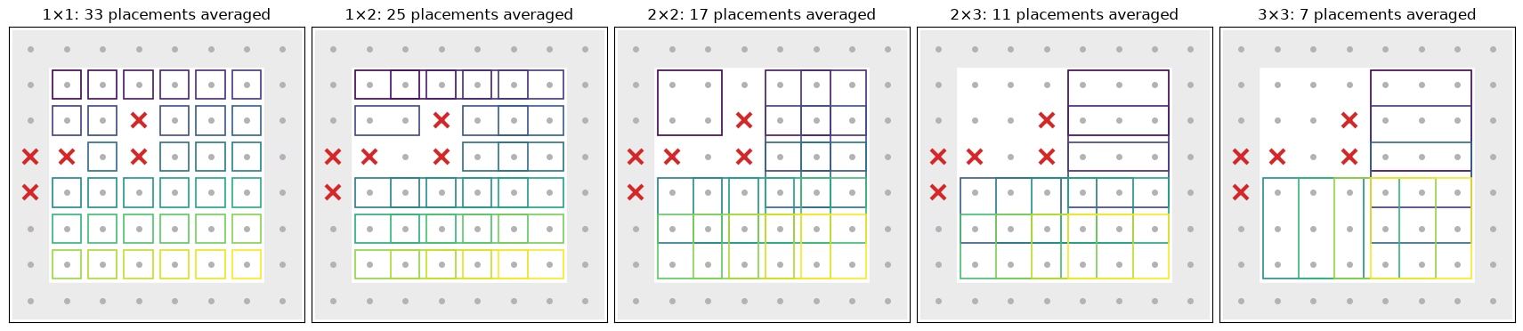
כלל שמשתמש רק בנתונים: qubit נחשב פגום אם ה-IPR של qubit בודד שלו ב- נמצא במרחק של עד מ-, הערך עבור qubit מעורבב לגמרי. מאחר שה-IPR של qubit אחד הוא , זה מסמן qubits עם . שוליים שמכילים אתר מסומן נשארים בחוץ בהמשך.
site_iprs = np.array(
    [
        ipr_from_shots(raw_bits[calibration_hw][0][:, :, [q]])
        for q in range(num_qubits_hw)
    ]
)
# |IPR - 1/2| < 0.25**2 / 2 is the same as |<Z>| < 0.25
flagged = {
    q for q in range(num_qubits_hw) if abs(site_iprs[q] - 0.5) < 0.25**2 / 2
}
print(
    f"Median single-qubit IPR at J0: {np.median(site_iprs):.2f}; flagged lattice sites {sorted(flagged)}"
)
Median single-qubit IPR at J0: 0.77; flagged lattice sites [19, 24, 25, 27, 32]
בחירת השוליים לחישוב הממוצע
התא הבא מראה אילו מיקומים של כל צורה נכנסים לממוצעים שלהלן: כל מיקום בתוך הסריג בלי אתר מסומן (איקסים אדומים). מיקומים שנוגעים בקצה (מוצללים) נשארים בחוץ. ל-qubits בקצה יש פחות קשרים, ולכן הם מתערבבים לאט יותר. כשמחשבים להם ממוצע בנפרד, הם חוצים צעד שלם של מאוחר יותר ממיקומים בתוך הסריג, לכל צורה ושיטה. לכל מיקום שנכנס לממוצע יש קופסה משלו, בצבע לפי המיקום.
def touches_edge(qubits):
    # Whether a placement includes a site on the edge of the lattice
    return any(
        q % num_cols_hw in (0, num_cols_hw - 1)
        or q // num_cols_hw in (0, num_rows_hw - 1)
        for q in qubits
    )

# The placements of each shape that enter the averages: in the bulk, and without a flagged site
kept_placements = {
    label: [
        k
        for k, qubits in enumerate(patch_list)
        if not touches_edge(qubits) and not set(qubits) & flagged
    ]
    for label, patch_list in positions.items()
}
placement_cmap = plt.get_cmap("viridis")
fig, axes = plt.subplots(
    1, len(positions), figsize=(17, 4.4), layout="constrained"
)
for ax, (label, patch_list) in zip(axes, positions.items()):
    width, height = patch_shapes[label]
    for q in range(num_qubits_hw):
        x, y = q % num_cols_hw, q // num_cols_hw
        if touches_edge([q]):  # shade the edge of the lattice
            ax.add_patch(
                plt.Rectangle(
                    (x - 0.5, y - 0.5), 1, 1, color="0.92", zorder=0
                )
            )
        ax.plot(x, y, "o", color="0.7", ms=4, zorder=1)
    kept = kept_placements[label]
    for i, k in enumerate(kept):
        qubits = patch_list[k]
        x0, y0 = (
            qubits[0] % num_cols_hw,
            qubits[0] // num_cols_hw,
        )  # top-left site of the placement
        ax.add_patch(
            plt.Rectangle(
                (x0 - 0.4, y0 - 0.4),
                width - 0.2,
                height - 0.2,
                fill=False,
                lw=1.2,
                ec=placement_cmap(i / max(len(kept) - 1, 1)),
                zorder=2,
            )
        )
    for q in flagged:
        ax.plot(
            q % num_cols_hw,
            q // num_cols_hw,
            "x",
            color="#d62728",
            ms=11,
            mew=3,
            zorder=3,
        )
    ax.set_xlim(-0.6, num_cols_hw - 0.4)
    ax.set_ylim(num_rows_hw - 0.4, -0.6)
    ax.set_aspect("equal")
    ax.set_xticks([])
    ax.set_yticks([])
    ax.set_title(f"{label}: {len(kept)} placements averaged")
plt.show()
PEA
השיטה השלישית אינה צריכה הפניה קלאסית. לכל זוגיות, לוקחים את הערכים בגורמי רעש 1, 1.5 ו-2, מחלקים בדיכוי הקריאה שנלמד (TREX), מתאימים אקספוננט בגורם הרעש ומבצעים אקסטרפולציה לרעש אפס. זוגיות שמחליפות סימן או קרובות לאפס מקבלות התאמת קו ישר. הפחתת השונות דורשת אומדן אמין שלה, וזה קל עבור זוגיות גולמיות ומוגדלות, אך לא עבור הפלט של התאמה לא ליניארית עם חיתוך וחלופות. לכן PEA משתמשת בדרך הסטנדרטית האחרת להסרת ההטיה של ריבוע. מבצעים אקסטרפולציה לכל מחצית מהאקראיזציות בנפרד ומכפילים את שני האומדנים הבלתי תלויים.
def readout_fidelity(support):
    # Damping of <Z_S> by the learned readout noise
    pauli = QubitSparsePauli.from_sparse_label(
        ("Z" * len(support), list(support)), num_qubits_hw
    )
    return readout_map.pauli_fidelity(pauli)

def extrapolate_to_zero(values):
    # Fit a * exp(b * factor) to each column of values (noise factors first), or a line
    # where the values change sign or come within 1e-3 of zero
    result = np.polynomial.polynomial.polyfit(noise_factors, values, 1)[0]
    sign = np.sign(values[0])
    usable = np.all(np.sign(values) == sign, axis=0) & (
        np.abs(values).min(axis=0) > 1e-3
    )
    if usable.any():
        log_fit = np.polynomial.polynomial.polyfit(
            noise_factors, np.log(np.abs(values[:, usable])), 1
        )
        result[usable] = sign[usable] * np.exp(log_fit[0])
    return result

def pea_ipr(parities, fidelities, num_patch):
    # parities has shape (noise factors, randomizations, supports). Extrapolate the two
    # halves of the randomizations separately; their errors are independent, so the
    # product of the two estimates of each parity has no shot-noise bias
    def zero_noise(p):
        # A parity cannot exceed 1 in magnitude, so cap the extrapolated values there
        return np.clip(
            extrapolate_to_zero(p.mean(axis=1) / fidelities), -1, 1
        )

    half = parities.shape[1] // 2
    first, second = (
        zero_noise(parities[:, :half]),
        zero_noise(parities[:, half:]),
    )
    return float((1 + np.dot(first, second)) / 2**num_patch)
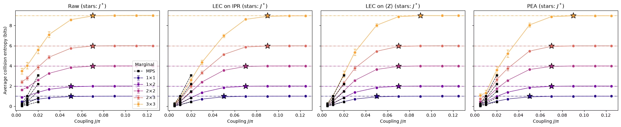
כל ארבעת האומדנים, והמעברים
הפונקציה הבאה מחשבת את האומדנים הגולמי, LEC על IPR, LEC על ו-PEA של ה-IPR של מיקום שוליים אחד בכל צימוד. היא גם מעריכה את רעש ה-shots של כל אחד, באמצעות bootstrapping של האקראיזציות. התא מריץ אותה לכל מיקום שנכנס לממוצעים, מה שנמשך כדקה וחצי.
def estimate_iprs(qubits, key):
    # Raw, LEC-on-IPR, LEC-on-<Z>, and PEA IPRs of one marginal position at every coupling,
    # with the shot noise of each from a bootstrap over the randomizations
    n = len(qubits)
    supports = parity_supports(qubits)
    # Parities with shape (noise factors, randomizations, supports), per coupling
    parities = [
        np.stack([parity_expectation_values(b, supports) for b in bits])
        for bits in raw_bits
    ]
    patch_bits = [
        bits[0][:, :, qubits] for bits in raw_bits
    ]  # noise factor 1
    values, errors = lec_estimates(
        patch_bits,
        [p[0] for p in parities],
        references[(calibration_hw, 64)][key],
        calibration_hw,
        n,
    )
    fidelities = np.array([readout_fidelity(s) for s in supports])

    def pea_statistic(p):
        return pea_ipr(p, fidelities, n)

    values["raw"] = [ipr_from_shots(b) for b in patch_bits]
    errors["raw"] = [bootstrap_error(ipr_from_shots, b) for b in patch_bits]
    values["PEA"] = [pea_statistic(p) for p in parities]
    errors["PEA"] = [
        bootstrap_error(pea_statistic, p, axis=1) for p in parities
    ]  # randomizations are axis 1
    return {m: np.array(v) for m, v in values.items()}, {
        m: np.array(e) for m, e in errors.items()
    }

methods = ["LEC on IPR", "LEC on ⟨Z⟩", "PEA"]
method_colors = {
    "LEC on IPR": "#2a78d6",
    "LEC on ⟨Z⟩": "#1baf7a",
    "PEA": "#eb6834",
}
iprs, ipr_errors = {}, {}
for label, patch_list in positions.items():
    for k in kept_placements[label]:
        iprs[label, k], ipr_errors[label, k] = estimate_iprs(
            patch_list[k], f"{label} {k}"
        )
print(f"{len(iprs)} clean marginal positions")
93 clean marginal positions
def crossover_coupling(couplings, entropies, haar, tolerance=0.1):
    # Smallest coupling whose entropy is within tolerance of the random-state value
    for coupling, entropy in zip(couplings, entropies):
        if entropy >= haar - tolerance:
            return coupling
    return None

def reference_ipr(index, chi, key):
    # IPR of the MPS distribution of a marginal
    return float((references[(index, chi)][key] ** 2).sum())

mps_settings = [
    (calibration_hw, 64),
    (1, 128),
    (2, 128),
]  # (coupling index, bond dimension)
panels = ["raw", *methods]

# Average IPR of every shape over its clean placements, then the entropy and the crossover
hw_entropies = {
    method: {} for method in panels
}  # per method and shape: average entropy and its error
crossovers = {method: {} for method in panels}
mps_entropies = {}  # per shape: MPS entropy, averaged over the same placements, at mps_settings
for label, patch_list in positions.items():
    haar = haar_entropy(len(patch_list[0]), num_qubits_hw)
    keys = [(shape, k) for (shape, k) in iprs if shape == label]
    mps_entropies[label] = [
        collision_entropy(
            np.mean([reference_ipr(j, chi, f"{label} {k}") for _, k in keys])
        )
        for j, chi in mps_settings
    ]
    for method in panels:
        ipr, ipr_error = average_ipr(
            [iprs[key][method] for key in keys],
            [ipr_errors[key][method] for key in keys],
        )
        entropy = collision_entropy(ipr)
        hw_entropies[method][label] = (entropy, ipr_error / (ipr * np.log(2)))
        crossovers[method][label] = crossover_coupling(
            couplings_hw, entropy, haar
        )
fig, axes = plt.subplots(
    1, len(panels), figsize=(5 * len(panels), 4.2), sharey=True
)
for (label, patch_list), color in zip(positions.items(), colors):
    haar = haar_entropy(len(patch_list[0]), num_qubits_hw)
    for ax, method in zip(axes, panels):
        entropy, error = hw_entropies[method][label]
        ax.errorbar(
            couplings_hw / np.pi,
            entropy,
            yerr=error,
            fmt="o-",
            color=color,
            mec="white",
            ms=7,
            lw=1,
            capsize=3,
            label=label,
        )
        ax.plot(
            couplings_hw[[j for j, _ in mps_settings]] / np.pi,
            mps_entropies[label],
            "s--",
            color="black",
            ms=4,
            lw=1,
            label="MPS" if label == "3×3" else None,
            zorder=4,
        )
        ax.axhline(haar, color=color, ls="dashdot", lw=0.9)
        if crossovers[method][label]:
            ax.plot(
                crossovers[method][label] / np.pi,
                haar,
                "*",
                ms=14,
                color=color,
                mec="black",
                zorder=3,
            )
for ax, method in zip(axes, panels):
    ax.set_title(f"{'Raw' if method == 'raw' else method} (stars: $J^*$)")
    ax.set_xlabel("Coupling $J/\\pi$")
axes[0].set_ylabel("Average collision entropy (bits)")
axes[0].legend(title="Marginal", loc="lower right")
fig.tight_layout()
plt.show()
סיכום
מה נדרש כדי להריץ ניסוי בגודל כזה:
-
מעגלים שמבנהם אינו תלוי ב-, שמקומפלים תת-שכבה אחת בכל פעם, כך שמודל רעש אחד משרת את כל הסריקה.
-
אומדנים שעובדים ממחרוזות ביטים: ספירת זוגות עבור ה-IPR של שוליים, והצורה של Parseval, עם הפחתת השונות מכל זוגיות מוגדלת בריבוע, כשהקלט הוא ערכי תצפית אחרי mitigation.
-
עוגן קלאסי זול: המצב האידיאלי ב- קטן מכייל את הרעש, וצימודים מוחזקים בצד בודקים את הכיול. כיול של כל בנפרד, ולא של ה-IPR כולו, הוא מה שגורם לשוליים הגדולים להתאים.
-
כלי IBM לעבודה הכבדה: קופסאות ו-twirling של Samplomatic,
NoiseLearnerV3, dynamical decoupling, ו-job אחד שלExecutorעם הגברת רעש עבור PEA. -
בדיקות איכות נתונים שמשתמשות רק בנתונים.
השלבים הבאים. כדי להמשיך עם mitigation, ראו את המדריכים הגברת שגיאות הסתברותית ו-PEC עם lightcones מוצללים.